Summary
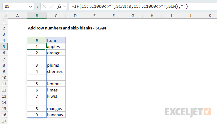
To add sequential row numbers to a list of data, skipping cells that are blank, you can use the SCAN function with a trim reference. In the example shown, the formula in B5 is:
=IF(C5:.C1000<>"",SCAN(0,C5:.C1000<>"",SUM),"")
The result is a running count that numbers each item in column C and skips the empty rows. When items are added to the list, the numbers extend automatically. Trim references are available in Excel 365 only. For a formula that works in any version of Excel, copy this formula down the column:
=IF(C5<>"",SUMPRODUCT(--($C$5:C5<>"")),"")
Both formulas also work when the list is created by formulas that return empty strings. See below for details.
Generic formula
=IF(range<>"",SCAN(0,range<>"",SUM),"")
Explanation
In the example shown, the goal is to add row numbers in column B only when there is a value in column C. Rows with a value should be numbered in order, and empty rows should be skipped. This article explains two formulas that follow the same logic: if a cell isn't empty, return a count of the non-empty cells so far. In Excel 365, a single formula based on the SCAN function numbers the whole list at once. In any version of Excel, a formula based on the SUMPRODUCT function can be copied down the column instead.
Row numbers with SCAN
In Excel 365, the easiest way to number the items in a list and skip blank rows is to generate a running count with the SCAN function. The formula in B5 is:
=IF(C5:.C1000<>"",SCAN(0,C5:.C1000<>"",SUM),"")
C5:.C1000 is a trim reference: the dot after the colon tells Excel to trim empty rows from the end of the range. The last item is in cell C16, so the range becomes C5:C16. Blank rows inside the list are not trimmed.
Working from the inside out, the expression C5:.C1000<>"" tests each cell, returning TRUE for cells that contain a value and FALSE for cells that are empty:
{TRUE;TRUE;FALSE;TRUE;TRUE;FALSE;TRUE;TRUE;TRUE;FALSE;TRUE;TRUE}
SCAN works through this array one value at a time, starting at zero. At each step, SUM adds the current value to the running total, counting TRUE as 1 and FALSE as 0, so the count goes up at each item and stays the same at each blank row:
{1;2;2;3;4;4;5;6;7;7;8;9}
SUM is given by name, without a LAMBDA, which is a shortcut called an eta lambda. Finally, the IF function runs the same test again. Where a cell has a value, IF returns the running count. Otherwise, IF returns an empty string (""):
{1;2;"";3;4;"";5;6;7;"";8;9}
This array lands in cell B5 and spills into the range B5:B16. When an item is added below the list, the trimmed range grows, and a new number appears. If the list is completely empty, the trim reference returns a #REF! error.
Row numbers in any version of Excel
In any version of Excel, you can number the list with a formula copied down the column. In the worksheet below, the formula in B5 is:
=IF(C5<>"",SUMPRODUCT(--($C$5:C5<>"")),"")
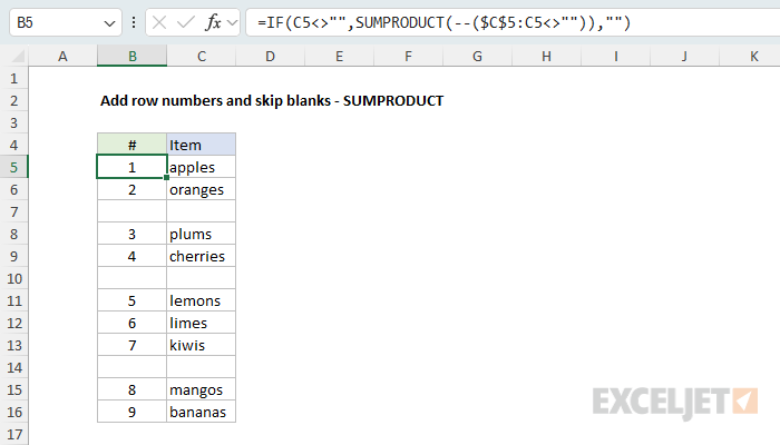
This formula uses the same logic as the SCAN formula above, one row at a time. The IF function first checks if cell C5 has a value. If not, IF returns an empty string (""). You can also use LEN(C5) as the test, which returns zero for an empty cell or an empty string. If C5 has a value, IF returns a count of the non-empty cells from C5 down to the current row:
SUMPRODUCT(--($C$5:C5<>""))
$C$5:C5 is an expanding reference: the first cell is locked and the second is not, so the range grows by one row each time the formula is copied down. The expression $C$5:C5<>"" returns TRUE for each cell in the range that contains a value, the double negative (--) converts TRUE and FALSE to 1 and 0, and SUMPRODUCT adds up the result. In row 8, for example, the range is C5:C8, and the count is 3.
Why not use the COUNTA function to count the values? COUNTA works fine when the values are typed in. But if the list is created by formulas that return an empty string ("") when there is nothing to display, COUNTA counts those cells too, because they contain a formula. The empty rows are skipped, but the numbers jump: 1, 2, 4, 5, 7, and so on. The test <>"" treats an empty string like an empty cell, so the SUMPRODUCT formula numbers both kinds of list correctly.
Why SUMPRODUCT instead of SUM? In Excel 2021+ and Excel 365, SUM(--($C$5:C5<>"")) returns the same result. In older versions of Excel, SUM needs to be entered with Control + Shift + Enter to evaluate the array; entered normally, it returns 1 in every numbered row. SUMPRODUCT handles arrays natively in every version. For more, see Why SUMPRODUCT?
Note: a cell that contains a space character is not empty, so both formulas will number a row that contains only a space.