Summary
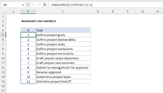
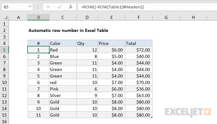
To add automatic row numbers to an Excel Table, you can use a formula based on the ROW function. In the example shown, the formula in B5, copied down, is:
=ROW()-ROW(Table1[#Headers])
Note: The table name is not required. However, Excel will add the table name automatically if omitted.
Generic formula
=ROW()-ROW([#Headers])
Explanation
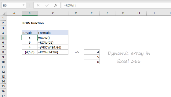
When no argument is provided, the ROW function returns the "current row", that is, the row number of the cell that contains it. When a cell reference is provided, ROW returns the row number of the cell. When a range is provided, ROW returns the first row number in the range.
In the example shown, the formula in B5 is:
=ROW()-ROW(Table1[#Headers])
The first ROW returns 5, since ROW is provided no argument, and resides in cell B5. The second ROW uses a structured reference:
Table1[#Headers] // header row
The header row resolves to the range $B$4:$F$4, so ROW returns 4. For the first 3 rows of the table, we have:
B5=5-4 // 1
B6=6-4 // 2
B7=7-4 // 3
No header row
The formula above works great as long as a table has a header row, but it will fail if the header row is disabled. If you are working with a table without a header row, you can use this alternative:
=ROW()-INDEX(ROW(Table1),1,1)+1
In this formula, the first ROW function returns the current row, as above. The INDEX function returns the first cell in the range Table1 (cell B5) to the second ROW function, which always returns 5. For the first 3 rows of the table, the formula works like this:
B5=5-5+1 // 1
B6=6-5+1 // 2
B7=7-5+1 // 3
This formula will continue to work normally even when the header row is disabled.