Summary
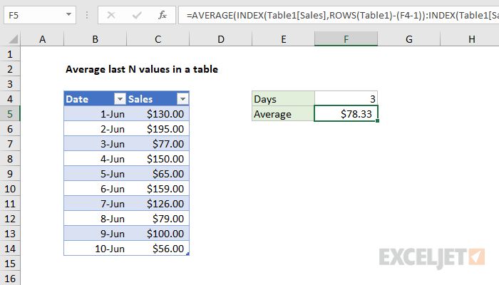
To calculate the average for the last N values n an Excel table (i.e. last 3 rows, last 5 rows, etc.) you can use the AVERAGE function together with the INDEX and ROWS functions. In the example shown, the formula in F5 is:
=AVERAGE(INDEX(Table1[Sales],ROWS(Table1)-(F4-1)):INDEX(Table1[Sales],ROWS(Table1)))
Generic formula
=AVERAGE(INDEX(table[column],ROWS(table)-(N-1)):INDEX(table[column],ROWS(table)))
Explanation
This formula is a good example of how structured references can make working with data in Excel much easier. At the core, this is what we're doing:
=AVERAGE(first:last)
where "first" is a reference to the first cell to include in the average and "last" is a reference to the last cell to include. The result is a range that includes the N cells to average.
To get the first cell in the range, we use INDEX like this:
INDEX(Table1[Sales],ROWS(Table1)-(F4-1))
The array is the entire Sales column, and row number worked by subtracting (n-1) from total rows.
In the example, F4 contains 3, so the row number is 10-(3-1) = 8. With a row number of 8, INDEX returns C12.
To get the last cell we use INDEX again like this:
INDEX(Table1[Sales],ROWS(Table1))
There are 10 rows in the table, so INDEX returns C14.
The AVERAGE function then returns the average of C12:C14, which is $78.33.