Sequence of leap years

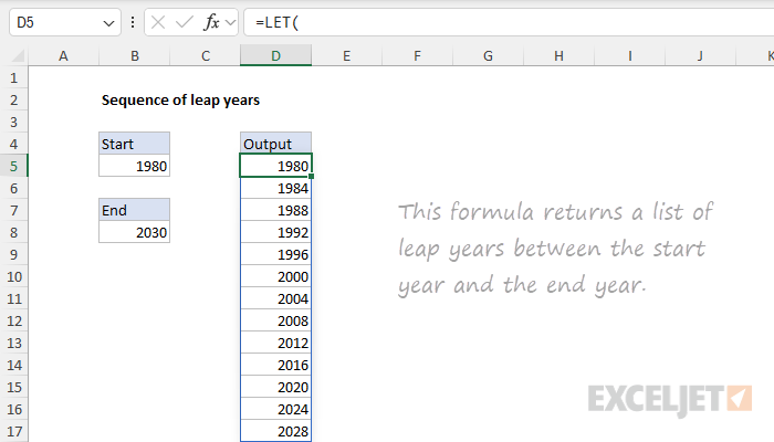
In this example, the goal is to generate the list of leap years between a given start year and end year. The worksheet is set up so that the start year is an input in cell B5 and the end year is an input in cell B8. If either value changes, the formula should generate a new list of leap years. In the current version of Excel, the easiest way to do this is with the SEQUENCE function and the FILTER function in a formula like this:

=LET(
start,B5,
end,B8,
years,SEQUENCE(end-start+1,,start),
leaps,(MOD(years,400)=0)+((MOD(years,4)=0)*(MOD(years,100)<>0)),
FILTER(years,leaps))

At a high level, this formula uses the SEQUENCE function to generate a list of all years between the start and end. Then it checks for leap years using logic implemented with the MOD function and filters out all non-leap years. At the start, the LET function defines four variables:

• start - the start year entered in cell B5
• end - the end year entered B8
• years - a sequence of all years between the start and end year
• leaps - a logical test that flags all leap years

Using LET this way keeps the formula efficient and readable. For example, the calculation for years (see below) only runs one time, even though it is used four times in the formula.

Generating a list of years

The next step in solving this problem is to generate a complete list of all years between the start and end year. We can do this with the SEQUENCE function, which is designed to create numeric arrays. For example, to generate the numbers 1 through 10 you can use SEQUENCE like this:

=SEQUENCE(10) // returns {1;2;3;4;5;6;7;8;9;10}

To generate a list of numbers between a given start and end, we can use a generic pattern like this:

=SEQUENCE(end-start+1,,start)

With the start year given as 1980 and the end year given as 2030, we have:

=SEQUENCE(end-start+1,,start)
=SEQUENCE(2030-1980+1,,1980)
=SEQUENCE(50+1,,1980)
=SEQUENCE(51,,1980)

The result is an array with the 51 years between 1980 and 2020, inclusive:

{1980;1981;1982;1983;1984;1985;1986;1987;1988;1989;1990;1991;1992;1993;1994;1995;1996;1997;1998;1999;2000;2001;2002;2003;2004;2005;2006;2007;2008;2009;2010;2011;2012;2013;2014;2015;2016;2017;2018;2019;2020;2021;2022;2023;2024;2025;2026;2027;2028;2029;2030}

This array is then assigned to the years variable defined by LET.

Testing for leap years

The next step is to test each year in years to identify leap years. This is done with the following snippet:

(MOD(years,400)=0)+((MOD(years,4)=0)*(MOD(years,100)<>0))

This logic here is based on the following leap year rule, which is explained in detail on this page:

To be a leap year, the year number must be divisible by four – except for end-of-century years, which must be divisible by 400. This means that 2000 is a leap year, but 1700, 1800, and 1900 are not leap years.

The test is implemented with Boolean algebra and the MOD function as follows:

1. If the year is divisible by 400, it's a leap year (TRUE).
2. Or if the year is divisible by 4 and not divisible by 100, it's a leap year (TRUE)
3. Otherwise, the year is not a leap year (FALSE).

The result is an array of 51 TRUE and FALSE values. The TRUE values in this array correspond to leap years in the original years array, and the FALSE values indicate non-leap years. The array is assigned to the leaps variable defined by LET.

Removing the non-leap years

The final step is removing non-leap years, which is done with the FILTER function like this:

FILTER(years,leaps)

Recall that the two arrays, years and leaps, are the same size; each array contains 51 rows. The FILTER function uses the leaps array to filter out non-leap years. The final result is an array that contains only leap years. This array lands in cell D5 and spills down the worksheet. If the values for start (B5) or end (B8) are changed, the entire process is repeated and a new list of leap years is generated.

Pro-tip: implement AND and OR

The formula above uses Boolean algebra to test for leap years, a compact yet cryptic way to apply conditions based on AND and OR logic. However, if you look at the formula explained here (which tests a single year) you'll notice that it uses the AND function and the OR function instead:

=OR(MOD(A1,400)=0,AND(MOD(A1,4)=0,MOD(A1,100)<>0))

Can we use this same approach here? We can, but we need to adjust the formula first. AND and OR are "aggregating functions", which means they return a single aggregated result. This won't work in this case, because we are running a test on 51 years and we need to get 51 results back in a single array so FILTER can use the array to remove non-leap years. The solution is to implement the AND and OR inside the BYROW function like this:

=LET(
start,B5,
end,B8,
years,SEQUENCE(end-start+1,,start),
leaps,BYROW(years,LAMBDA(y,OR(MOD(y,400)=0,AND(MOD(y,4)=0,MOD(y,100)<>0)))),
FILTER(years,leaps))

In this version, leaps is defined with BYROW like this:

BYROW(years,LAMBDA(y,OR(MOD(y,400)=0,AND(MOD(y,4)=0,MOD(y,100)<>0))))

BYROW processes values in a row-by-row fashion, so each year (defined as y above) is tested separately. The result for each year is a single TRUE or FALSE value. The BYROW function packages the results into a single array, which we hand off to FILTER as before.