Summary
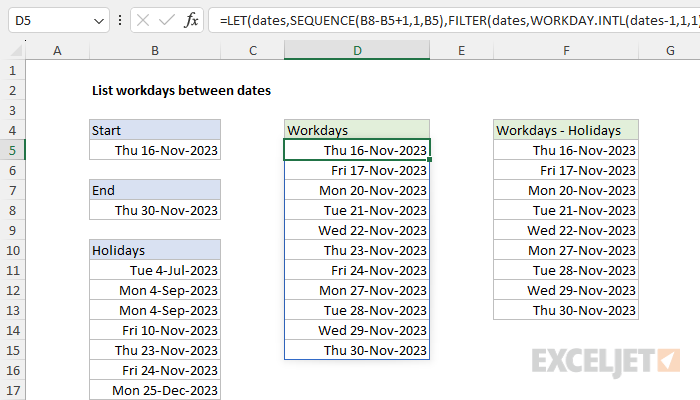
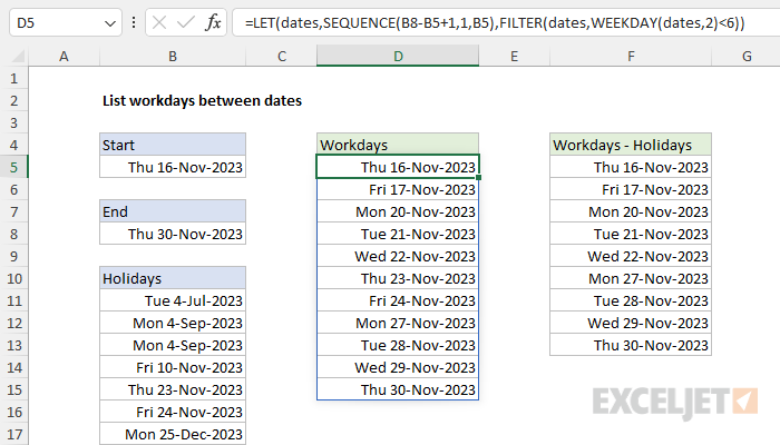
To list the workdays between two dates you can use a formula based on the SEQUENCE function and the FILTER function. In the worksheet shown, the formula in cell D5 is:
=LET(dates,SEQUENCE(B8-B5+1,1,B5),FILTER(dates,WORKDAY.INTL(dates-1,1,1)=dates))
The result in cell D5:D15 is the eleven workdays between 16-Nov-2023 and 30-Nov-2023, inclusive. Note that this list excludes weekends (Saturday and Sunday) but does not exclude holidays. See below for a version of the formula that excludes holidays.
Generic formula
=LET(dates,SEQUENCE(end-start+1,1,start),FILTER(dates,WEEKDAY(dates,2)<6))
Explanation
The goal is to list the working days between a start date and an end date. In the simplest form, this means we want to list dates that are Monday, Tuesday, Wednesday, Thursday, or Friday, but exclude dates that are Saturday or Sunday. In addition, we need an option to exclude a list of given holidays. This article describes two ways to approach this problem, both of which use the SEQUENCE function to "spin up" a full range of dates and the FILTER function to remove dates that are not working days. Both methods also use the LET function to name and store the array from SEQUENCE so that it can be reused later in the formula.
The difference is that the first method uses the WORKDAY.INTL function to test dates as working days whereas the second method uses a more transparent manual approach to logically filter dates with the WEEKDAY and XMATCH functions. The second method is presented mainly as an example of how dynamic array formulas in Excel can be adapted to solve many different problems. Finally note that although the workbook shown is used to list workdays over just a two-week period, the approach will work to list workdays over much larger time frames, for example, 3 months, 6 months, 1 year, etc.
Note: In the workbook shown, all dates use the custom number format "ddd d-mmm-yyyy". This date format is used to make it easy to see the day of the week along with the date.
Creating the dates
Both methods below use the SEQUENCE function to create an array of dates that cover the entire date range. SEQUENCE is designed to generate numeric sequences in rows and/or columns. The generic syntax for SEQUENCE looks like this:
=SEQUENCE(rows,[columns],[start],[step])
In this example, the goal is to generate a series of dates that span the date range defined by the start date in cell B5 and the end date in cell B8, inclusive. We use SEQUENCE to generate the dates like this:
SEQUENCE(B8-B5+1,1,B5)
The arguments inside SEQUENCE have the following values:
- rows - B8-B5+1 (45260-45246+1 = 15)
- columns = 1
- start - B5 (45246)
Note: Dates in Excel are large serial numbers.
After Excel evaluates the arguments, we can simplify the formula to this:
SEQUENCE(15,1,45246)
The SEQUENCE function then creates an array of 15 dates starting at 45246 (16-Nov-2023). The result is an array like this:
{45246;45247;45248;45249;45250;45251;45252;45253;45254;45255;45256;45257;45258;45259;45260}
These serial numbers represent the 15 dates between 16-Nov-2023 and 30-Nov-2023, inclusive. Inside the main formula, the LET function defines the array above as the variable dates. The FILTER function is then used to remove non-working days from dates, using one of the two methods explained below.
Method 1
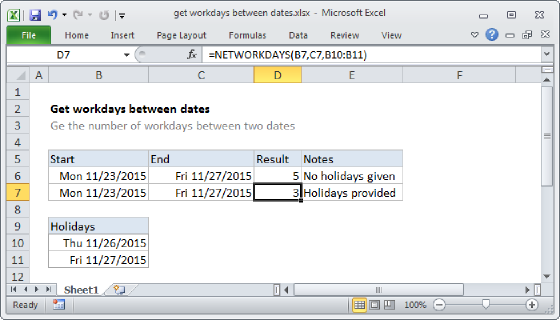
The first method relies on the WORKDAY.INTL function to test dates as working days. This approach builds on the Date is workday formula here. The WORKDAY.INTL function is an upgraded version of the older WORKDAY function.
WORKDAY.INTL function
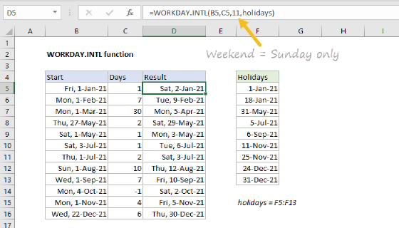
The WORKDAY.INTL function takes a date and returns the next workday based on a given offset value provided as the days argument. WORKDAY.INTL will automatically exclude weekends (Saturday and Sunday) and can optionally exclude dates that are holidays. The generic syntax for WORKDAY.INTL looks like this:
=WORKDAY.INTL(start_date,days,[weekend],[holidays])
The arguments inside WORKDAY.INTL have the following purpose:
- start_date - the date to start from
- days - the number of days to move forward or back
- weekend - the weekend scheme to use
- holidays - dates to be excluded as holidays
The screen below shows the basic operation of WORKDAY.INTL:
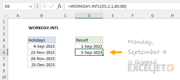
As you can see above, we are starting on September 1, 2023 (Friday) and asking for the next workday 1 day forward in the calendar. WORKDAY.INTL skips Saturday and Sunday because we are using the default value (1) weekend and also skips Monday, September 4, 2023, because that date is listed as a holiday in the range B5:B8. That is the basic operation of WORKDAY.INTL. For more details, see How to use the WORKDAY.INTL function.
In the worksheet shown at the top of the page in cell D5, we use WORKDAY.INTL like this:
=LET(dates,SEQUENCE(B8-B5+1,1,B5),FILTER(dates,WORKDAY.INTL(dates-1,1,1)=dates))
As explained above, the SEQUENCE function is used to generate an array that contains all dates between 16-Nov-2023 and 30-Nov-2023, inclusive, and the LET function stores the result in dates:
=LET(dates,SEQUENCE(B8-B5+1,1,B5)
Next the WORKDAY.INTL function is used with the FILTER function to remove non-working days:
FILTER(dates,WORKDAY.INTL(dates-1,1,1)=dates)
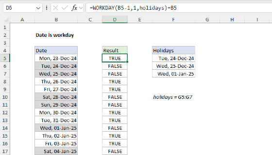
This is the tricky part of the formula. It builds on the Date is workday formula here. The WORKDAY.INTL function does not allow you to test a date with a "zero offset". In other words, you can't test a single date by providing the date with 0 for days. However, you can "step back" 1 day in time and check the "next day" with a value of 1 for days. Then you can compare the result to the day you want to test. If they are the same, you know you have a workday. If they are different, you know you have a non-working day. Although slightly non-intuitive, this is the trick we use in the formula:
WORKDAY.INTL(dates-1,1,1)=dates
For start_date in WORKDAY.INTL, we subtract 1 from dates, which results in an array of "day before" values. Then we ask WORKDAY.INTL for the "next workday" using the altered values. Finally, we compare the results from WORKDAY.INTL with the original dates. In the example shown, the result is an array of 15 TRUE and FALSE values like this:
{TRUE;TRUE;FALSE;FALSE;TRUE;TRUE;TRUE;TRUE;TRUE;FALSE;FALSE;TRUE;TRUE;TRUE;TRUE}
Each value in this array tells us whether a date is a working day or not for the 15 days in the date range between 16-Nov-2023 and 30-Nov-2023. Finally, the FILTER function uses this array to filter out non-working days. The final result that lands in cell D5 is this array:
{45246;45247;45250;45251;45252;45253;45254;45257;45258;45259;45260}
These are the 11 working days in the date range between 16-Nov-2023 and 30-Nov-2023.
Exclude Holidays
The formula above can be easily extended to exclude holidays as well. The formula in F5 looks like this:
=LET(dates,SEQUENCE(B8-B5+1,1,B5),FILTER(dates,WORKDAY.INTL(dates-1,1,1,B11:B17)=dates))
This version of the formula adds the holidays that appear in the range B11:B17 to the WORKDAY.INTL function, which then excludes November 23 and 24 from the results listed in F5:F13.
Method 2
Another way to solve this problem is to use more basic functions in Excel to filter out non-working days. The main reason to take this approach is to build a more transparent formula that can apply custom logic not provided by WORKDAY.INTL. For example, you could check and exclude dates using more than one list of holidays. The explanation below shows how to solve the same problem using a combination of the WEEKDAY function and the XMATCH function instead of WORKDAY.INTL.
List workdays
To list all days between two dates while excluding Saturday and Sunday, you can use a formula like this in cell D5:
=LET(dates,SEQUENCE(B8-B5+1,1,B5),FILTER(dates,WEEKDAY(dates,2)<6))
First, the LET function is used to define the dates variable with the SEQUENCE function like this:
=LET(dates,SEQUENCE(B8-B5+1,1,B5)
The inputs to SEQUENCE are as follows:
- rows - B8-B5+1 (the count of days, which is 15 in the workbook shown)
- columns - 1 (defaults to 1 and could be omitted)
- start - the date in B5 (16-Nov-2023, or 45246 in serial number format)
The result from SEQUENCE is an array of 15 dates in serial number format like this:
{45246;45247;45248;45249;45250;45251;45252;45253;45254;45255;45256;45257;45258;45259;45260}
These numbers represent all dates between 16-Nov-2023 and 30-Nov-2023, inclusive. This array is then assigned to the variable dates by the LET function. Next, the dates are run through the FILTER function to remove Saturdays and Sundays:
FILTER(dates,WEEKDAY(dates,2)<6)
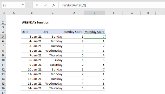
The logic used to filter out weekends is defined by the WEEKDAY function here:
WEEKDAY(dates,2)<6
The serial_number argument is given as dates from the previous step. Return_type is provided as 2. WEEKDAY returns a number for each day of the week. By default, WEEKDAY will return numbers that correspond to a Sunday-based week where Sunday is 1, Monday is 2, Tuesday is 3, and so on. Providing 2 for return_type tells WEEKDAY to return numbers that correspond to a Monday-based week. In this scheme, Monday is 1, Tuesday is 2, Wednesday is 3, etc. By testing for weekdays that are less than 6, we are effectively filtering out Saturdays (6) and Sundays (7). After FILTER runs, the result is the eleven workdays seen in the range D5:D15. Note that this version of the formula does not exclude holidays. See below for an option that does.
Remove holidays
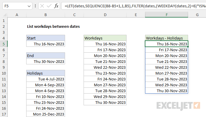
So far, we have a working formula that excludes Saturdays and Sundays but does not exclude holidays. To exclude holidays, we need to extend the logic inside the FILTER function to remove dates that are holidays. To do this, the formula used in cell F5 looks like this:
=LET(dates,SEQUENCE(B8-B5+1,1,B5),FILTER(dates,(WEEKDAY(dates,2)<6)*ISNA(XMATCH(dates,B11:B17))))
This formula is the same as the formula explained above except that the logic used inside FILTER has been extended to check for holidays like this:
(WEEKDAY(dates,2)<6)*ISNA(XMATCH(dates,B11:B17))
Notice that the first part of this expression is the same as above; we are using WEEKDAY to remove Saturdays and Sundays. The second part of the expression uses the XMATCH function to test for holidays like this:
ISNA(XMATCH(dates,B11:B17))
Essentially, we are looking up each date in dates in the range B11:B17, which contains dates that are holidays with the XMATCH function. If XMATCH finds a match (i.e. the date is a holiday) it will return a number representing the position of the match. If XMATCH does not find a match (the date is not a holiday) it will return the #N/A error. Consequently, we use the ISNA function to test for an #N/A error. IF ISNA returns TRUE, it means the date is not a holiday. If ISNA returns FALSE, the date is a holiday.
Notice the WEEKDAY expression and the ISNA function are joined with a multiplication operator (*). This is an example of Boolean algebra. Effectively, it joins the two expressions with AND logic, so both must be true. When the include argument inside FILTER is evaluated, the math operation converts the TRUE and FALSE values to 1s and 0s:
=FILTER(dates,{1;1;0;0;1;1;1;1;1;0;0;1;1;1;1}*{1;1;1;1;1;1;1;0;0;1;1;1;1;1;1})
The result after multiplication looks like this:
=FILTER(dates,{1;1;0;0;1;1;1;0;0;0;0;1;1;1;1})
The 1s in the array represent dates that are working days (not Saturday or Sunday and not a holiday). The 0s represent dates that are a Saturday a Sunday or a holiday. Only the dates associated with 1s make it through FILTER. Notice the final result starting in cell F5 contains nine dates (2 less than the previous formula) because 2 dates in the date range are holidays.
Cleaned up formula
Since we are already using the LET function, we can clean things up a bit like this:
=LET(
start,B5,
end,B8,
holidays,B11:B17,
dates,SEQUENCE(end-start+1,1,start),
FILTER(dates,(WEEKDAY(dates,2)<6)*ISNA(XMATCH(dates,holidays))))
In this version, we define the needed cell references and variables at the top. This makes the remaining code below more generic and easier to read.