Summary
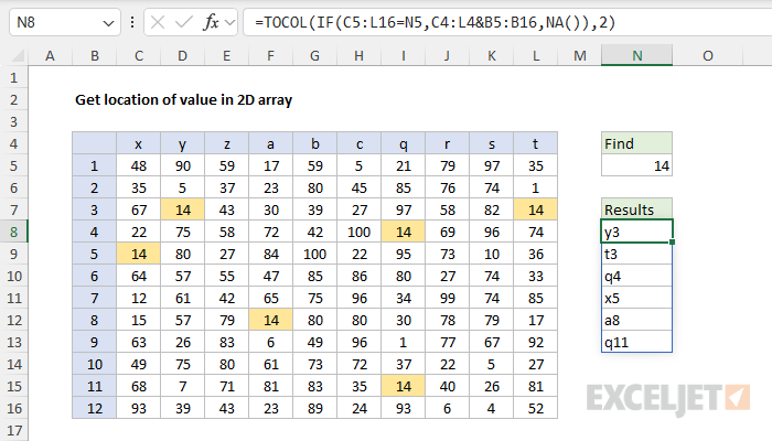
To find the coordinates of all matching values in a 2D array you can use a formula based on the IF function and the TOCOL function. In the worksheet shown, the formula in cell N8 is:
=TOCOL(IF(C5:L16=N5,C4:L4&B5:B16,NA()),2)
When the formula is entered, it returns the coordinates of each cell that contains the value entered in cell N5, using the values in row 4 and column B for coordinates. If the value in N5, or if the range C5:L16 are updated, the the formula will return a new set of results. This formula can be adjusted to return Excel cell addresses, as explained below.
Generic formula
=TOCOL(IF(data=A1,range1&range2,NA()),2)
Explanation
In this example, the goal is to return a list of the locations for a specific value in a 2D array of values (i.e., a table). The target value is entered in cell N5, and the table being tested is in the range C4:L16. The coordinates are supplied from row 4 and column B, as seen in the worksheet. In the current version of Excel, which supports dynamic array formulas, an easy way to solve this problem is with the IF function together with the TOCOL function. Although this example shown is generic, you can adapt a formula like this to perform a variety of tasks, including:
- Track the location of specific items in a warehouse.
- List open seats in a venue or classroom.
- Show the location of items on a game board.
- Find open time slots in a schedule grid.
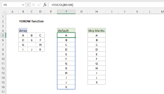
The TOCOL function is a new function in Excel designed to flatten 2D arrays into a single column. By default, TOCOL will scan values by row, but it can also scan values by column. In addition, TOCOL can be configured to optionally ignore errors, a feature we use in this example.
Conditional formatting to highlight matches
Although it is not needed to list matched locations, the worksheet shown in the example is configured to highlight the value in N5 wherever it appears with a conditional formatting rule applied to the range C5:L16. This makes it easy to see at a glance where matching values are located. To create a rule like this:
- Select the range C5:L16.
- Home > Conditional Formatting > New rule.
- Use a formula to determine which cells to format.
- Enter the formula "=C5=$N$5" in the input area.
- Select the formatting of your choice.
- Click OK to save the rule.
Returning arbitrary coordinates
In the worksheet shown above, we are returning a set of coordinates based on the values entered in row 4 and column B. These values are arbitrary and can be customized as desired. In the worksheet shown, the formula in cell N8 is:
=TOCOL(IF(C5:L16=N5,C4:L4&B5:B16,NA()),2)
Working from the inside out, the core of this formula is based on the IF function, which is configured like this:
IF(C5:L16=N5,C4:L4&B5:B16,NA())
- logical_test - C5:L16=N5
- value_if_true - C4:L4&B5:B16
- value_if_false - NA()
The key to understanding this operation is to remember that we are testing 120 values in the table (12 rows x 10 columns), which means the IF function will return 120 results. The IF function evaluates each value in C5:L1 against the value in N5 and returns a single array with 120 TRUE/FALSE values like this:
{FALSE,FALSE,FALSE,FALSE,FALSE,FALSE,FALSE,FALSE,FALSE,FALSE;FALSE,FALSE,FALSE,FALSE,FALSE,FALSE,FALSE,FALSE,FALSE,FALSE;FALSE,TRUE,FALSE,FALSE,FALSE,FALSE,FALSE,FALSE,FALSE,TRUE;FALSE,FALSE,FALSE,FALSE,FALSE,FALSE,TRUE,FALSE,FALSE,FALSE;TRUE,FALSE,FALSE,FALSE,FALSE,FALSE,FALSE,FALSE,FALSE,FALSE;FALSE,FALSE,FALSE,FALSE,FALSE,FALSE,FALSE,FALSE,FALSE,FALSE;FALSE,FALSE,FALSE,FALSE,FALSE,FALSE,FALSE,FALSE,FALSE,FALSE;FALSE,FALSE,FALSE,TRUE,FALSE,FALSE,FALSE,FALSE,FALSE,FALSE;FALSE,FALSE,FALSE,FALSE,FALSE,FALSE,FALSE,FALSE,FALSE,FALSE;FALSE,FALSE,FALSE,FALSE,FALSE,FALSE,FALSE,FALSE,FALSE,FALSE;FALSE,FALSE,FALSE,FALSE,FALSE,FALSE,TRUE,FALSE,FALSE,FALSE;FALSE,FALSE,FALSE,FALSE,FALSE,FALSE,FALSE,FALSE,FALSE,FALSE}
The TRUE values indicate a match, and the FALSE values indicate non-matching cells. Inside the value_if_true argument, the expression "C4:L4&B5:B16" joins the values in C4:L4 to the values in B5:B16 using concatenation. The result is an array of 120 coordinates, one for each cell in the table:
{"x1","y1","z1","a1","b1","c1","q1","r1","s1","t1";"x2","y2","z2","a2","b2","c2","q2","r2","s2","t2";"x3","y3","z3","a3","b3","c3","q3","r3","s3","t3";"x4","y4","z4","a4","b4","c4","q4","r4","s4","t4";"x5","y5","z5","a5","b5","c5","q5","r5","s5","t5";"x6","y6","z6","a6","b6","c6","q6","r6","s6","t6";"x7","y7","z7","a7","b7","c7","q7","r7","s7","t7";"x8","y8","z8","a8","b8","c8","q8","r8","s8","t8";"x9","y9","z9","a9","b9","c9","q9","r9","s9","t9";"x10","y10","z10","a10","b10","c10","q10","r10","s10","t10";"x11","y11","z11","a11","b11","c11","q11","r11","s11","t11";"x12","y12","z12","a12","b12","c12","q12","r12","s12","t12"}
As IF works through the results, it returns the associated coordinate for each TRUE created by the logical test. For FALSE results, IF uses the NA function to return a #N/A error. The result from IF is an array that contains 120 results, one for each cell in the table:
{#N/A,#N/A,#N/A,#N/A,#N/A,#N/A,#N/A,#N/A,#N/A,#N/A;#N/A,#N/A,#N/A,#N/A,#N/A,#N/A,#N/A,#N/A,#N/A,#N/A;#N/A,"y3",#N/A,#N/A,#N/A,#N/A,#N/A,#N/A,#N/A,"t3";#N/A,#N/A,#N/A,#N/A,#N/A,#N/A,"q4",#N/A,#N/A,#N/A;"x5",#N/A,#N/A,#N/A,#N/A,#N/A,#N/A,#N/A,#N/A,#N/A;#N/A,#N/A,#N/A,#N/A,#N/A,#N/A,#N/A,#N/A,#N/A,#N/A;#N/A,#N/A,#N/A,#N/A,#N/A,#N/A,#N/A,#N/A,#N/A,#N/A;#N/A,#N/A,#N/A,"a8",#N/A,#N/A,#N/A,#N/A,#N/A,#N/A;#N/A,#N/A,#N/A,#N/A,#N/A,#N/A,#N/A,#N/A,#N/A,#N/A;#N/A,#N/A,#N/A,#N/A,#N/A,#N/A,#N/A,#N/A,#N/A,#N/A;#N/A,#N/A,#N/A,#N/A,#N/A,#N/A,"q11",#N/A,#N/A,#N/A;#N/A,#N/A,#N/A,#N/A,#N/A,#N/A,#N/A,#N/A,#N/A,#N/A}
If you look closely, you can see 6 matched locations floating in a sea of #N/A errors. These correspond to cells in B5:L16 that contain the same value as N5. The entire array is delivered to the TOCOL function, which is configured like this:
=TOCOL(IF(...),2)
- array - result from the IF function
- ignore - 2, to ignore errors
Now you can see why we've configured TOCOL to ignore all errors; we only want to keep values associated with matches, discarding the #N/A errors in the process. The result from TOCOL is a single array that contains six coordinates:
{"y3";"t3";"q4";"x5";"a8";"q11"}
This array lands in cell N8 and spills into the range N8:N14. If the value in N5 or the values in B5:L16 are changed, the formula will return new results. The coordinates in C4:L4 and B5:B16 can be customized as desired.
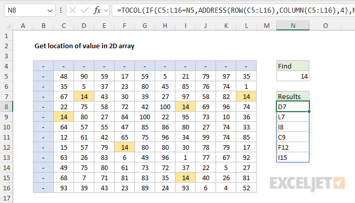
Returning cell addresses
In the example above, the goal is to return (arbitrary) coordinates entered in C4:L4 and B5:B16. The idea is that you can customize these values as needed to support your particular use case. However, you might also want to return Excel native cell addresses. To do that, you can use a modified version of the formula that adds the ADDRESS function like this:
=TOCOL(IF(C5:L16=N5,ADDRESS(ROW(C5:L16),COLUMN(C5:L16),4),NA()),2)
The overall structure and flow of this formula are the same as the original explained above: IF tests each value and returns the locations of matching cells, and the TOCOL function removes the errors and stacks the remaining values in a column:
IF(C5:L16=N5,ADDRESS(ROW(C5:L16),COLUMN(C5:L16),4),NA())
- logical_test - C5:L16=N5
- value_if_true - ADDRESS(ROW(C5:L16),COLUMN(C5:L16),4)
- value_if_false - NA()
The difference is in the value_if_true argument, which uses the ADDRESS function to create an address for each matching value with help from the ROW function and the COLUMN function:
ADDRESS(ROW(C5:L16),COLUMN(C5:L16),4)
- row_num - ROW(C5:L16)
- column_num - COLUMN(C5:L16)
- abs_num - 4, for relative address format
After IF runs, it returns an array of results (mostly errors) to TOCOL:
=TOCOL({#N/A,#N/A,#N/A,#N/A,#N/A,#N/A,#N/A,#N/A,#N/A,#N/A;#N/A,#N/A,#N/A,#N/A,#N/A,#N/A,#N/A,#N/A,#N/A,#N/A;#N/A,"D7",#N/A,#N/A,#N/A,#N/A,#N/A,#N/A,#N/A,"L7";#N/A,#N/A,#N/A,#N/A,#N/A,#N/A,"I8",#N/A,#N/A,#N/A;"C9",#N/A,#N/A,#N/A,#N/A,#N/A,#N/A,#N/A,#N/A,#N/A;#N/A,#N/A,#N/A,#N/A,#N/A,#N/A,#N/A,#N/A,#N/A,#N/A;#N/A,#N/A,#N/A,#N/A,#N/A,#N/A,#N/A,#N/A,#N/A,#N/A;#N/A,#N/A,#N/A,"F12",#N/A,#N/A,#N/A,#N/A,#N/A,#N/A;#N/A,#N/A,#N/A,#N/A,#N/A,#N/A,#N/A,#N/A,#N/A,#N/A;#N/A,#N/A,#N/A,#N/A,#N/A,#N/A,#N/A,#N/A,#N/A,#N/A;#N/A,#N/A,#N/A,#N/A,#N/A,#N/A,"I15",#N/A,#N/A,#N/A;#N/A,#N/A,#N/A,#N/A,#N/A,#N/A,#N/A,#N/A,#N/A,#N/A},2)
As before, TOCOL is configured to ignore errors, and the final result is a single array with six matching cell addresses like his:
{"D7";"L7";"I8";"C9";"F12";"I15"}
The ADDRESS function can optionally return absolute addresses or R1C1-style addresses by adjusting the abs_num argument. For details, see our ADDRESS function page.
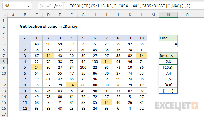
Returning numeric coordinates in brackets
The worksheet below shows another way to return numeric coordinates, this time using a "[1,1]" syntax relative to the table of values. The formula in cell N8 has been modified like this:
=TOCOL(IF(C5:L16=N5,"["&C4:L4&","&B5:B16&"]",NA()),2)
Here again, we use concatenation to assemble numeric coordinates in square brackets when a cell matches the value in N5:
"["&C4:L4&","&B5:B16&"]"
Otherwise, the formula's structure is the same. You can see the result below:
If you are new to the concept of concatenation, see: How to concatenate in Excel.
Note: In the worksheet above, the numeric coordinates are manually entered in C4:L4 and B5:B16. However, the formula could easily be adjusted to use the SEQUENCE function to automatically create numeric sequences to match the size of any table.
MAP function alternative
Because I'm always on the lookout for good MAP function examples, I want to mention that you can also use MAP to solve a problem like this. The equivalent formula for the first example explained above is:
=TOCOL(MAP(C5:L16,C4:L4&B5:B16,LAMBDA(a,b,IF(a=N5,b,NA()))),2)
Although MAP requires a custom LAMBDA calculation, it also provides a framework to separate the logic in the formula into discrete parts. In addition, because MAP iterates through values individually, you can combine MAP with functions like AND and OR. Normally, this is not possible with arrays because AND and OR are aggregate functions that return a single result.
TEXTJOIN alternative
If you only want a list of coordinates as a text string (i.e., you don't want individual results in separate cells), you can use the TEXTJOIN function in a formula like this:
=TEXTJOIN(", ",1,IF(C5:L16=N5,C4:L4&B5:B16,""))
Here, we configure IF to return empty strings ("") instead of #N/A errors, and then we configure TEXTJOIN to ignore empty values and join the coordinates together, separated by a comma and a space (", ").
Note: TOCOL does not ignore empty strings ("") in the same way as TEXTJOIN, which is why the TOCOL formula is based on ignoring errors. I'm not sure why this is. It would be better if TOCOL also ignored empty strings in formulas. Let me know if you notice this changing at some point in the future!