Summary
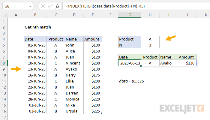
To get the nth matching record in a set of data, you can use the FILTER function with the INDEX function. In the example shown, the formula in cell G8 is:
=INDEX(FILTER(data,data[Product]=H4),H5)
Where data is an Excel Table in the range B5:E16. When H4 contains "A" and H5 contains 3, the result will be the 3rd record in the table where the product is "A".
Generic formula
=INDEX(FILTER(range,logical_test),n)
Explanation
The goal is to retrieve the nth matching record in a set of data, after filtering on a specific product. In the worksheet shown, the product in H4 and the value for n in H5 are inputs that can be changed at any time. For instance, if the product in H4 is "A" and the value in H5 is 3, the formula should return the 3rd record in the table where the product is "A", as shown in the screen above. This can be accomplished with the FILTER function and the INDEX function.
FILTER function
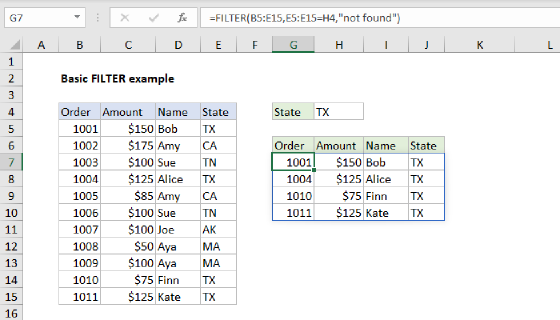
The FILTER function "filters" data based on a logical test and extracts matching records. The generic syntax for FILTER looks like this:
=FILTER(array,include,[if_empty])
The array is the data to filter, and the include argument is the logical expression to use when filtering. The if_empty parameter specifies the value to return if no matches are found. Note that by itself, FILTER returns all matching data. For example, if we configure FILTER to match on product "A", it will extract all 5 matching records as seen below:
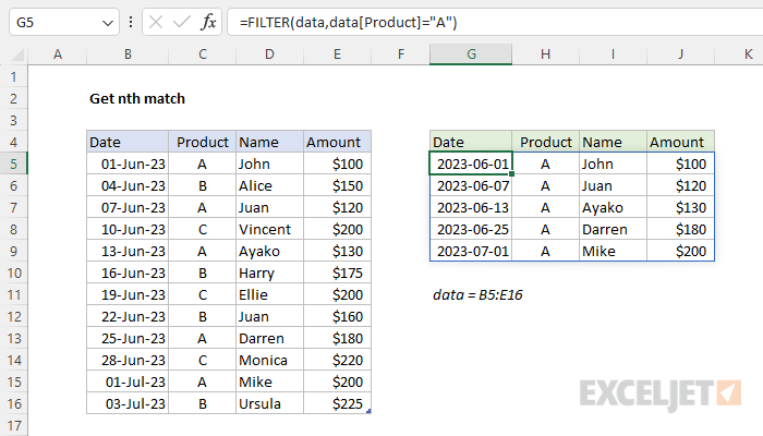
To just return the nth record from this data, we need another function.
INDEX function
=INDEX(FILTER(data,data[Product]="A",n)
The INDEX function returns the value at a given location in a range or array. You can use INDEX to retrieve individual values, or entire rows and columns. The generic syntax for INDEX looks like this:
=INDEX(array,row_num,[col_num])
In this case, we only need to provide a row number to get back the nth match returned by FILTER. To get the 3rd match for product "A", we nest the FILTER function inside INDEX for array, then supply 3 for row_num:
=INDEX(FILTER(data,data[Product]="A"),3)
To complete the formula as shown, we need to replace the hard-coded reference for product and column number with H4 and H5:
=INDEX(FILTER(data,data[Product]=H4),H5)
Now when a different product is entered in cell H4, or a different value for n is entered in cell H5, the formula will return a new result.
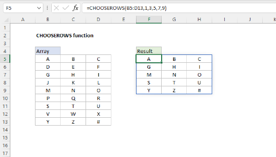
CHOOSEROWS function
The CHOOSEROWS function, a more recent addition to Excel, is designed to return one or more rows from a range or array. As an alternative to INDEX, we can use the CHOOSEROWS function to solve this problem like this:
=CHOOSEROWS(FILTER(data,data[Product]=H4),H5)
This formula returns the same result as the INDEX version above.
Older versions of Excel
In older versions of Excel without the FILTER function, you can use a more complicated formula like this:
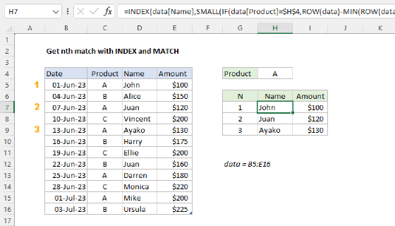
=INDEX(data,SMALL(IF(data[Product]=H4,ROW(data)-MIN(ROW(data))+1),H5),0)
This is an array formula and must be entered with Control + Shift + Enter in Excel 2019 and older.
The generic form of this formula looks like this:
=INDEX(rng,SMALL(IF(rng=value,ROW(rng)-MIN(ROW(rng))+1),n)
The core of this formula is the SMALL function, which returns the nth smallest value in an array of numeric values. In this case, the array provided to SMALL represents row numbers created with this part of the formula:
IF(data[Product]=H4,ROW(data)-MIN(ROW(data))+1)
Essentially, IF applies a filter based on the product in cell H4, then returns the corresponding row number from an array of row numbers created with this code:
ROW(list)-MIN(ROW(list))+1
Because the table contains 12 rows of data, the result is an array like this:
{1;2;3;4;5;6;7;8;9;10;11;12}
See this page for a full explanation of the code to create row numbers in Legacy Excel. Putting it all together, SMALL returns the 3rd smallest row number that corresponds with "A" products:
SMALL(IF(data[Product]=H4,{1;2;3;4;5;6;7;8;9;10;11;12}),H5)
With "A" in cell H4, the result is 5. Simplifying, the original formula becomes:
=INDEX(data,5,0)
And INDEX returns row 5 from the data. Note: (1) in older versions of Excel, the zero for col_num is required to return an entire row of data. (2) To display the entire row, enter the formula as a multi-cell array formula across all 4 cells simultaneously.