Summary
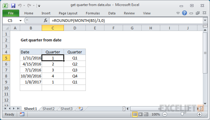
To calculate the quarter (i.e. 1,2,3,4) for a given date, you can use the ROUNDUP function together with the MONTH function. In the example shown, the formula in cell C5 is:
=ROUNDUP(MONTH(B5)/3,0)
The result is 1 since January 31 is in the first quarter.
This formula returns a standard quarter, where Q1 begins in December. See this formula to get a fiscal quarter.
Generic formula
=ROUNDUP(MONTH(date)/3,0)
Explanation
In this example, the goal is to return a number that represents quarter (i.e. 1,2,3,4) for any given date. In other words, we want to return the quarter that the date resides in.
ROUNDUP formula solution
In the example shown, the formula in cell C5 is:
=ROUNDUP(MONTH(B5)/3,0)
The ROUNDUP function works like the ROUND function, except that ROUNDUP will always round numbers 1-9 up to a given number of digits, supplied as the num_digits argument. In this case, because we want to get back an integer, we use zero for num_digits.
Working from the inside out, the MONTH function first extracts the month as a number between 1-12, then divides this number by 3:
=MONTH(B5)/3
=1/3
=0.3333
The result is then rounded up to the nearest whole number using the ROUNDUP function:
=ROUNDUP(0.3333,0) returns 1
The result is 1, since 0.3333 rounded up to the next whole number is 1.
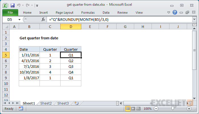
Adding "Q"
If you want the quarter number to include a "Q" you can concatenate the numeric result from ROUNDUP to the "Q". The formula in D5 is:
="Q"&ROUNDUP(MONTH(B5)/3,0) // returns "Q1"
The result is the letter "Q" prepended to the number: