Summary
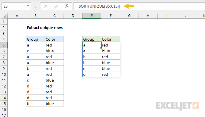
To extract a list of unique rows from a set of data, you can use the UNIQUE function together with the SORT function. In the example shown, the formula in E5 is:
=SORT(UNIQUE(B5:C15))
which return the 6 unique rows in the range B5:C15, sorted by group.
Generic formula
=SORT(UNIQUE(range))
Explanation
In this example, the goal is to extract a list of unique rows from the range B5:C15. The easiest way to do this is to use the UNIQUE function.
By default, UNIQUE will extract unique values in rows, so there is no special configuration needed. Working from the inside out, we give UNIQUE the full range of data, including the Group and Color columns:
UNIQUE(B5:C15)
The UNIQUE function evaluates all 11 rows and returns the 6 unique rows in an unsorted two-dimensional array that looks like this:
{"a","red";"c","blue";"a","blue";"b","red";"d","red";"b","blue"}
This array is returned directly to the SORT function:
=SORT({"a","red";"c","blue";"a","blue";"b","red";"d","red";"b","blue"})
By default, SORT will sort based on the first column in the data. The result is the same array, sorted by Group:
{"a","red";"a","blue";"b","red";"b","blue";"c","blue";"d","red"}
UNIQUE is a dynamic function. If any data in B5:C15 changes, the output from UNIQUE will update immediately.
Dynamic source range
UNIQUE won't automatically adjust the source range if data is added or deleted. To give UNIQUE a range that will automatically resize as needed, use an Excel Table or create a dynamic named range with a formula.