Summary
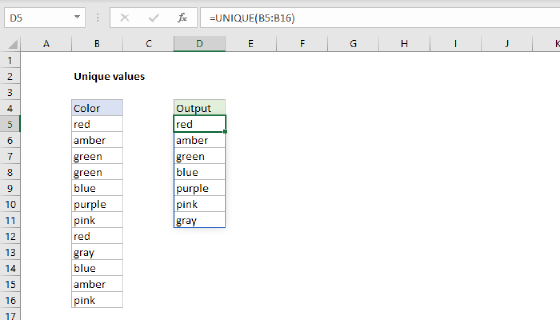
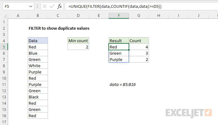
To list duplicate values in a set of data based on a threshold count, you can use a formula based on FILTER, UNIQUE, and the COUNTIF function. In the example shown, the formula in F5 is:
=UNIQUE(FILTER(data,COUNTIF(data,data)>=D5))
This formula lists the duplicate values in the named range data (B5:B16) using the "Min count" value in D5 as a minimum threshold. In other words, a value must occur in the data at least as many times as the number in D5. The result from the formula is dynamic and will change if the number in D5 is changed.
Explanation
In this example, the goal is to list and count values that are duplicated in a set of data at least n times, where n is provided as a variable in cell D5. All data is in the named range data (B5:B16). In the worksheet shown, the formula used in cell F5 is:
=UNIQUE(FILTER(data,COUNTIF(data,data)>=D5))
Working from the inside out, the first step is to count the values in data. This is done with the COUNTIF function like this:
COUNTIF(data,data) // get all counts
Because there are 12 values in data, and data is used for both range and criteria, COUNTIF returns an array with 12 counts as a result:
{4;1;3;1;2;4;2;3;1;4;3;4} // result from COUNTIF
Each number represents the count of one value in data. For example, because "Red" is the first value in data, and because "Red" occurs 4 times total, the first number in the array is 4. The next step is to compare these counts to the "Min count" in D5:
=COUNTIF(data,data)>=D5
={4;1;3;1;2;4;2;3;1;4;3;4}>=D5
Cell D5 contains 2, so the result is an array of 12 TRUE and FALSE values like this:
={TRUE;FALSE;TRUE;FALSE;TRUE;TRUE;TRUE;TRUE;FALSE;TRUE;TRUE;TRUE}
Each TRUE in this array represents a value that occurs at least 2 times in the data. This array is returned directly to the FILTER function as the include argument, and FILTER uses the array to return values that correspond to TRUE. These are values that occur at least twice in the data:
{"Red";"Green";"Purple";"Red";"Purple";"Green";"Red";"Green";"Red"}
FILTER returns the array to the UNIQUE function, and UNIQUE returns unique values:
{"Red";"Green";"Purple"}
These values spill into range F5:F7 as the final result. Notice each of these values occurs at least 2 times in data.
Summary count
To get the summary count seen in column G, the formula in G5 is:
=COUNTIF(data,F5#)
With data as range, and the spill range F5# as criteria, COUNTIF returns the count that each value in column F appears in data.
Dynamic source range
Because data (B5:B16) is a normal named range, it won't resize if data is added or deleted. To use a dynamic range that will automatically resize when needed, you can use an Excel Table, or create a dynamic named range with a formula.