Unique values by count

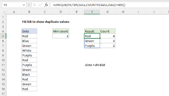
To extract a list of unique values from a set of data, filtered by count or occurrence, you can use UNIQUE with FILTER, and apply criteria with the COUNTIF function. In the example shown, the formula in D5 is:

=UNIQUE(FILTER(data,COUNTIF(data,data)>1))

which outputs the 3 unique values that appear more than once in the named range data (B5:B16).

Note: In this example, we are extracting a unique list of values that appear more than once. In other words, we are creating a list of duplicates :) The language is somewhat confusing.

Explanation

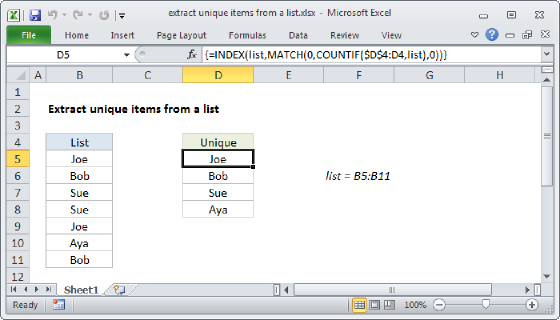
This example uses the UNIQUE function together with the FILTER function. You can see a more basic example here.

The trick in this case is to apply criteria to the FILTER function to only allow values based on count of occurence. Working from the inside out, this is done with COUNTIF and the FILTER function here:

FILTER(data,COUNTIF(data,data)>1)

The result from COUNTIF is an array of counts like this:

{3;1;3;3;2;1;1;3;1;2;3;3}

which are checked with the logical comparison > 1 to yield an array or TRUE/FALSE values:

{TRUE;FALSE;TRUE;TRUE;TRUE;FALSE;FALSE;TRUE;FALSE;TRUE;TRUE;TRUE}

Notice TRUE corresponds to values in the data that appear more than once. This array is returned to FILTER as the include argument, used to filter the data. FILTER returns another array as a result:

{"red";"green";"green";"blue";"red";"blue";"red";"green"}

This array is returned directly to the UNIQUE function as the array argument. Notice of the 12 original values, only 8 survive.

UNIQUE then removes duplicates, and returns the final array:

{"red";"green";"blue"}

If values in B5:B16 change, the output will update immediately.

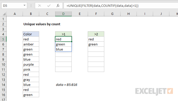
Count > 2

The formula in F5, which lists colors appearing at least 2 times in the source data, is:

=UNIQUE(FILTER(data,COUNTIF(data,data)>2))

Dynamic source range

Because data (B5:B15) is a normal named range, it won't resize if data is added or deleted. To use a dynamic range that will automatically resize when needed, you can use an Excel Table, or create a dynamic named range with a formula.