Summary
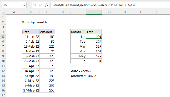
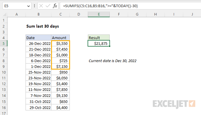
To sum values in the last 30 dates by date, you can use the SUMIFS function together with the TODAY function. In the example shown, the formula in E5, copied down, is:
=SUMIFS(C5:C16,B5:B16,">="&TODAY()-30)
The result is $21,875. This is the total of amounts in column C that occur in the last 30 days, based on a current date of December 30, 2022.
Generic formula
=SUMIFS(values,dates,">="&TODAY()-30)
Explanation
In this example, the goal is to calculate total amounts in column C that occur in the last 30 days, based on a current date of December 30, 2022. There are three basic approaches to solving this problem: (1) a traditional approach based on the SUMIFS function, (2) a more flexible approach that uses Boolean logic and the SUMPRODUCT function, a modern approach based on the FILTER function. Each approach is explained below.
Excel date logic
To understand the logic of the formulas explained below, the first step is to understand Excel's date system, where dates are serial numbers beginning on January 1, 1900. January 1, 1900 is 1, January 2, 1900 is 2, and so on. More recent dates are much larger numbers. For example, January 1, 1999 is 36161, January 1, 2010 is 40179, and January 1, 2020 is 43831. Because dates are just numbers, you can easily perform arithmetic on dates. For example, with January 1, 2020 in cell A1:
=A1+10 // Jan 11, 2020
=A1-10 // Dec 22, 2019
This also means we can use the TODAY function to return the current date, then subtract 30 days to get a date 30 days earlier. For example, as I write this, the current date is December 30, 2022 so:
=TODAY() // Dec 30, 2022
=TODAY()-30 // Nov 30, 2022
Therefore, to test if a date in cell A1 occurs within the last 30 days, we can use a formula like this:
=A1>=TODAY()-30
The above will return TRUE if the date is within the last 30 days of the current date and FALSE if not.
SUMIFS function
As mentioned above, the traditional way to solve a problem like this is to use the SUMIFS function. The SUMIFS function sums cells in a range that meet one or more conditions, referred to as criteria. To apply criteria, the SUMIFS function supports logical operators (>,<,<>,=) and wildcards (*,?) for partial matching. The generic syntax for SUMIFS looks like this:
=SUMIFS(sum_range,range1,criteria1) // 1 condition
where sum_range contains the values to sum, range is the cell range to test, and criteria1 is the criteria to apply to range. To solve this problem, we begin with the sum_range, which is C5:C16:
=SUMIFS(C5:C16,
Next, we add the range, which contains the dates in B5:B16:
=SUMIFS(C5:C16,B5:B16,
Finally, we add the criteria:
=SUMIFS(C5:C16,B5:B16,">="&TODAY()-30)
This is the tricky part of the formula because the operator must be enclosed in double quotes (">=") and concatenated to the TODAY function less 30. This is because the SUMIFS function is in a group of eight functions that split logical criteria into two parts. You can read more about the details of using logical operators with SUMIFS, see this page.
SUMPRODUCT function
Another way to solve this problem is with the SUMPRODUCT function and Boolean logic like this:
=SUMPRODUCT((B5:B16>=TODAY()-30)*C5:C16)
In this case, we are multiplying all values in C5:C16 by an expression designed to "zero out" values that should not be included in the final sum:
(B5:B16>=TODAY()-30)
The result from the expression above is an array of TRUE and FALSE values like this:
{TRUE;TRUE;TRUE;TRUE;TRUE;FALSE;FALSE;FALSE;FALSE;FALSE;FALSE;FALSE}
The TRUE values in this array represent dates that occur in the last 30 days, based on a current date of December 30, 2022 returned by the TODAY function. These are the first five dates in the data as shown.
Next, the array above is multiplied by the values in C5:C16. In Excel, TRUE and FALSE values are automatically coerced to 1s and 0s by any math operation, so the multiplication step converts the arrays above to ones and zeros. We can visualize this operation inside of SUMPRODUCT like this:
=SUMPRODUCT({1;1;1;1;1;0;0;0;0;0;0;0}*C5:C16)
After multiplication, we have just a single array:
=SUMPRODUCT({5550;7450;1000;725;7150;0;0;0;0;0;0;0})
Notice that values associated with dates that are not within the past 30 days have been "zeroed out". With just one array to process, SUMPRODUCT returns the sum of all items in the array: 21,875.
Note: Why would you use SUMPRODUCT instead of SUMIFS? The biggest reason is flexibility. Unlike SUMPRODUCT, SUMIFS requires a cell range; you can't use an array. This means SUMIFS won't work in formulas that need to manipulate values before conditional logic is applied.
FILTER function
In the latest version of Excel, you can solve this problem with the FILTER function like this:
=SUM(FILTER(C5:C16,B5:B16>=TODAY()-30,0))
In this formula, we use the same logic explained above to target dates in the past 30 days:
B5:B16>=TODAY()-30 // last 30 days
The expression above returns an array of TRUE and FALSE values like this:
{TRUE;TRUE;TRUE;TRUE;TRUE;FALSE;FALSE;FALSE;FALSE;FALSE;FALSE;FALSE}
And this array is used to filter the values in C5:C16. The result from FILTER is then returned directly to the SUM function:
=SUM({5550;7450;1000;725;7150})
SUM then returns a final result of 21,875.