Summary
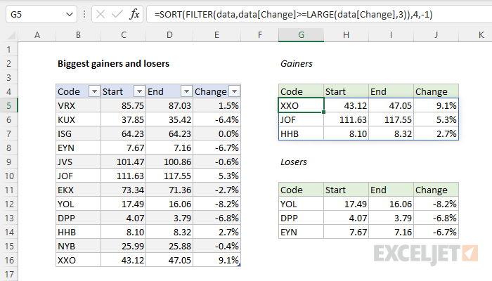
To list the top 3 gainers or losers from a set of data that contains a start and end value, you can use the FILTER function together with the LARGE and SMALL functions. In the example shown, the formula in G5 is:
=SORT(FILTER(data,data[Change]>=LARGE(data[Change],3)),4,-1)
where data is the Excel Table in B5:E16. A similar formula in G12 returns the 3 biggest losers. These results are dynamic and will immediately update if data changes. Read below for a detailed explanation of both formulas.
Note: Dynamic Array Formulas are only available in Excel 365 and Excel 2021.
Explanation
In this example, the goal is to display the biggest 3 gainers and losers in a set of data where Start and End columns contain values at two points in time, and Change contains the percentage change in the values. The data in B5:E16 is defined as an Excel Table with the name data. Two formulas are required, one to return the top 3 gainers in the table, and one to return the top 3 losers. The primary component of the solution is the FILTER function, which is used to extract data that meets specific logical conditions from the table.
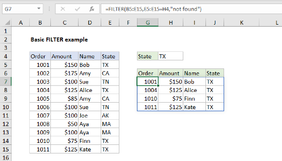
If you are new to FILTER, see this video: Basic FILTER function example
Top 3 gainers
In the example shown, the formula to return the top 3 gainers in cell G5 is:
=SORT(FILTER(data,data[Change]>=LARGE(data[Change],3)),4,-1)
Working from the inside out, the first task is to extract the three rows from the data that have the largest change values. To do this, we use the FILTER function together with the LARGE function like this:
FILTER(data,data[Change]>=LARGE(data[Change],3))
Inside FILTER, the array argument is the entire table, since we want to return all four columns. The include argument is a logical test based on the LARGE function:
data[Change]>=LARGE(data[Change],3)
The LARGE function is configured to return the third largest value in the Change column:
LARGE(data[Change],3) // get 3rd largest value
With 3 given for k, LARGE returns the 3rd largest value .02699 (2.699%). We can then simplify the FILTER function to the following:
FILTER(data,data[Change]>=0.0269)
Essentially, we are asking FILTER for rows in the table where change is greater than or equal to 0.0269. FILTER returns the 3 matching rows in an array like this:
{"JOF",111.63,117.546,0.053;
"HHB",8.104,8.323,0.0269;
"XXO",43.124,47.048,0.091}
Note: values have been rounded for readability.
At this point, we have the data we want, but it is not sorted. Since the goal is to show the biggest gainers first, we need to sort the array in descending order by Change. To do this, we use the SORT function directly on the array returned by FILTER:
=SORT(filtered_array,4,-1)
This is an example of nesting - the result from FILTER is delivered as an array inside the SORT function. Since the change column is the last column, sort_index is given as 4, and sort_index is provided as -1 to sort in descending order. Finally, the SORT function returns the final sorted array to cell G5, which spills into the range G5:J7.
Video: Basic SORT function example
Top 3 losers
Next, we need to list the biggest 3 losers. In the worksheet shown, the formula in G12 is:
=SORT(FILTER(data,data[Change]<=SMALL(data[Change],3)),4,1)
The first task is to extract the three rows from the data that have the smallest change values. To do this, we use the FILTER function together with the SMALL function like this:
FILTER(data,data[Change]<=SMALL(data[Change],3))
The array argument in FILTER is given as the table name data, since we want to return all four columns. The include argument is supplied as a logical expression that targets the three smallest values in Change:
data[Change]<=SMALL(data[Change]
The SMALL function returns the third largest change in the table:
SMALL(data[Change],3) // get 3rd smallest value
With 3 as k, SMALL returns -0.0671 (-6.7%). We can now simplify the FILTER function to this:
FILTER(data,data[Change]<=-0.0671)
We are asking FILTER for rows in data where Change is less than or equal to -0.0671. FILTER returns the 3 matching rows in an array like this:
{"EYN",7.673,7.158,-0.067;
"YOL",17.492,16.058,-0.082;
"DPP",4.067,3.790,-0.068}
Note: values have been rounded for readability.
We have the data we want, but it is unsorted. The goal is to show the biggest losers first, so we want to sort the array in ascending order by change. To do this, the FILTER function is nested inside the SORT function, and the result from FILTER is delivered as array:
=SORT(filtered_array,4,1)
Sort_index is given as 4, since change is the fourth column, and sort_index is provided as 1 because we want to sort ascending order, starting with the largest negative change. Finally, the SORT function returns the final sorted array to cell G12, which spills into the range G12:J14.
Note: this formula will always return the three rows in the data with the smallest change values, whether these values are negative or not. The label "losers" may not make sense in a small set of data with no negative change values.