Name of nth largest value

In a nutshell, this formula uses the LARGE function to find the nth largest value in a set of data. Once we have that value, we plug it into a standard INDEX and MATCH formula to retrieve the associated name. In other words, we use the nth largest value like a "key" to retrieve associated information.

The LARGE function is a straightforward way to get the nth largest value in a range. Simply provide a range for the first argument (array), and a value for n as the second argument (k):

 =LARGE(range,1) // 1st largest
 =LARGE(range,2) // 2nd largest
 =LARGE(range,3) // 3rd largest

Working from the inside out, the first step is to get the "1st" largest value in the data with the LARGE function:

LARGE(score,F5) // returns 93

In this case, the value in F5 is 1, so we are asking for the 1st largest score (i.e. the top score), which is 93. We can now simplify the formula to:

=INDEX(name,MATCH(93,score,0))

Inside the INDEX function, the MATCH function is set up to locate the position of 93 in the named range score (D5:D16):

MATCH(93,score,0) // returns 3

Since 93 appears in the 3rd row, MATCH returns 3 directly to INDEX as the row number, with name as array:

=INDEX(name,3) // Hannah

Finally, the INDEX function returns the name in the 3rd row, "Hannah".

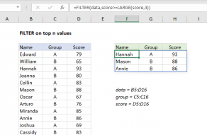
Notice we are picking up the values for n from the range F5:F7, in order to get the 1st, 2nd, and 3rd highest scores as the formula is copied down.

Retrieve group

The same basic formula will work to retrieve any associated information. To get the group for the largest values, you can simply change the array supplied to INDEX with the named range group:

=INDEX(group,MATCH(LARGE(score,F5),score,0))

With the value 1 in F5, LARGE will get the highest score, and the formula will return "A".

Note: with Excel 365, you can use the FILTER function to list top or bottom results dynamically.

With XLOOKUP

The XLOOKUP function can also be used to return the name of the nth largest value like this:

=XLOOKUP(LARGE(score,F5),score,name)

LARGE returns the largest value, 93, directly to XLOOKUP as the lookup value:

=XLOOKUP(93,score,name) //  Hannah

With the named range score (D5:D16) as the lookup array, and name (B5:B16) as the return array, XLOOKUP returns "Hannah" as before.

Handling ties

Duplicate values in the numeric data will create a "tie". If a tie occurs in the values being ranked, for example, if the first and second largest values are the same, LARGE will return the same value for each. When this value is passed into the MATCH function, MATCH will return the position of the first match, so you will see the same (first) name returned.

If there is the possibility of ties, you may want to implement some kind of tie-breaking strategy. One approach is to create a new helper column of values which have been adjusted to break ties. Then use the helper column values to rank and retrieve information. This makes the logic used to break ties clear and explicit.

Another approach is to break ties based on position only (i.e. the first tie "wins"). Here is a formula that takes that approach:

INDEX(name,MATCH(1,(score=LARGE(score,F5))*(COUNTIF(H$4:H4,name)=0),0))

Note: this is an array formula and must be entered with control + shift + enter, except in Excel 365.

Here, we use MATCH to find the number 1, and we construct a lookup array using boolean logic that (1) compares all scores to the value returned by LARGE:

score=LARGE(score,F5)

and (2) uses an expanding range check if the name is already in the ranked list:

COUNTIF(H$4:H4,name)=0

When a name is already in the list, it is "cancelled" by the logic, and the next (duplicate) value is matched. Notice the expanding range starts on the prior row, in order to avoid a circular reference.

This approach works in this example because there are no duplicate names in the name column. However, if duplicate names occur in ranked values, the approach needs to be adjusted. The easiest solution is to make sure that names are unique.

Notes

1. To get the name of nth value with criteria, (i.e. limit results to group A or B) you will need to extend the formula to use additional logic.
2. In Excel 365, the FILTER function is a better way to list top or bottom results dynamically. This approach will automatically handle ties.