Summary
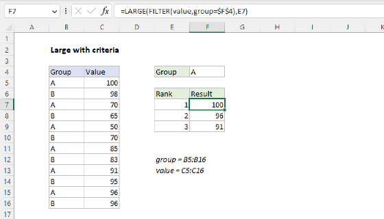
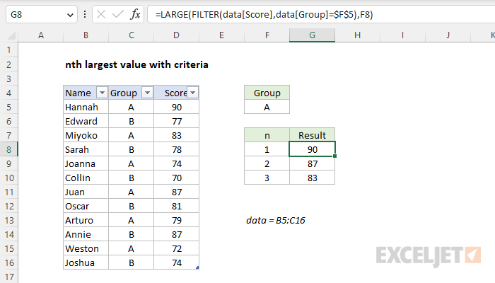
To return the nth largest value that meet specific conditions you can use a formula based on the LARGE function with the FILTER function. In the example shown, the formula in G8 is:
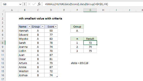
=LARGE(FILTER(data[Score],data[Group]=$F$5),F8)
where all data is in an Excel Table called data in the range B5:D16. As the formula is copied down, it returns the top 3 scores in group A, using the value in F5 ("A") for group and the value in column F for n.
Note: FILTER is a newer function in Excel. See below for a formula that will work in older versions.
Generic formula
=LARGE(FILTER(data,criteria),n)
Explanation
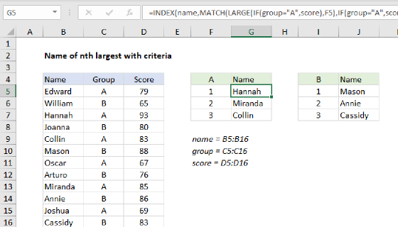
In this example, the goal is to retrieve the top 3 scores in column D that appear in a given group, entered as a variable in cell F5. If the group is changed, the formulas should calculate new results. The core of the solution is the LARGE function, which can be used to retrieve the "nth" largest value in a set of data. The challenge is that the LARGE function does not offer any built-in way to apply criteria before calculating a result. This means we need to create our own logic to apply criteria.
There are two basic ways to approach this problem. In the current version of Excel, you can use the FILTER function to apply conditions to data before it is delivered to LARGE. In older versions of Excel, you can use the IF function in an array formula. Both approaches are explained below.
Excel Table
For convenience, all data is in an Excel Table named data in the range B5:D16. Excel Tables are a convenient way to work with data in Excel because they (1) automatically expand to include new data and (2) offer structured references, which let you refer to data by name instead of by address. If you are new to Excel Tables, this article provides an overview. Also see this short video:
Video: How to create an Excel Table
LARGE function
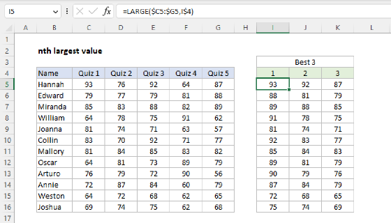
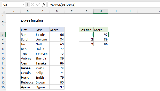
The LARGE function is used to return the nth largest value in a set of data like this:
=LARGE(range,n)
where n (k) is a number like 1, 2, 3, etc. For example, you can retrieve the first, second, and third largest values like this:
=LARGE(range,1) // first largest
=LARGE(range,2) // second largest
=LARGE(range,3) // third largest
The challenge in this problem is that LARGE has no built-in way to apply criteria. One way to apply criteria is with the FILTER function, as described in the next section.
LARGE with FILTER
In the current version of Excel, the FILTER function can be used to apply criteria inside of LARGE. This is the approach used in the worksheet shown, where the formula in G8 is:
=LARGE(FILTER(data[Score],data[Group]=$F$5),F8)
Working from the inside out, the FILTER function is configured to extract scores for the group in F5 like this:
FILTER(data[Score],data[Group]=$F$5)
Inside FILTER, array is given as the Score column, and the include argument is provided as an expression that compares each value in the Group column to the value in F5 ("A"). Note that $F$5 is an absolute reference, because we don't want this reference to change when the formula is copied down column G. Since there are 12 values in C5:C16, the expression returns an array with 12 TRUE and FALSE values like this:
{TRUE;FALSE;TRUE;FALSE;TRUE;FALSE;TRUE;FALSE;TRUE;FALSE;TRUE;FALSE}
The TRUE values indicate rows where the group equals "A". This array is used by FILTER to retrieve matching data. The result from FILTER is an array that contains the 6 values in group "A":
{90;83;74;87;79;72}
These values are provided to the LARGE function as the array argument. The second argument, k, comes from cell F8:
=LARGE({90;83;74;87;79;72},F8)
=LARGE({90;83;74;87;79;72},1)
=90
In cell G8, the result is 90, the (first) largest score in group A. As the formula is copied down, the value for k changes and LARGE returns the second and third best scores in group A.
LARGE with IF
In Legacy Excel, the FILTER function does not exist so we do not have a dedicated function to filter values by group. Instead, we can use a traditional array formula based on the IF function:
=LARGE(IF(data[Group]=$F$5,data[Score]),F8)
Note: this is an array formula and must be entered with control + shift + enter in Legacy Excel.
In this formula, the IF function serves the same purpose as the FILTER function above: it "filters" the values by group. Since we are running a logical test on 12 separate values in the Group column (C5:C16), we get an array that contains 12 results like this:
{90;FALSE;83;FALSE;74;FALSE;87;FALSE;79;FALSE;72;FALSE}
Notice that only values in group A make it into the array. The values in group B become FALSE when they fail the logical test. This array is returned directly to the LARGE function as the array argument. The value for k comes from cell F8:
=LARGE({90;FALSE;83;FALSE;74;FALSE;87;FALSE;79;FALSE;72;FALSE},F8)
=LARGE({90;FALSE;83;FALSE;74;FALSE;87;FALSE;79;FALSE;72;FALSE},1)
=90
LARGE automatically ignores the FALSE values and returns the largest number in the remaining values, which is 90. As the formula is copied down, the value for k changes and LARGE returns the second and third largest values in group A.
Multiple criteria
To apply multiple criteria, you can extend the formula with boolean logic. With FILTER, the generic formula looks like this:
=LARGE(FILTER(data,(criteria1)*(criteria2),n)
Where criteria1 and criteria2 are expressions to test specific conditions.
In older versions of Excel, you can use the same idea with the IF function like this:
=LARGE(IF((criteria1)*(criteria2),values),n)
For more information on using Boolean logic in array formulas, see the video below.