Summary
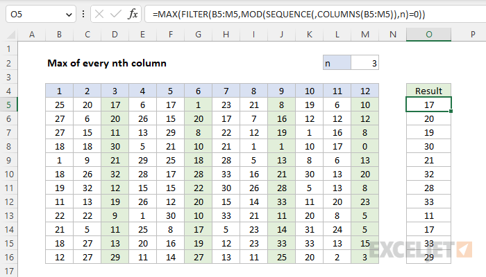
To get the max of every nth column, you can use a formula based on MAX, FILTER, MOD, SEQUENCE, and COLUMNS. In the example shown, the formula in O5 is:
=MAX(FILTER(B5:M5,MOD(SEQUENCE(,COLUMNS(B5:M5)),n)=0))
where n is the named range M2. With 3 in cell M2, the formula returns 17, the maximum value of the 3rd, 6th, 9th, and 12th values in B5:M5. If n is changed to another value, the formula will recalculate. See below for alternatives and a formula that will work in older versions of Excel.
Generic formula
=MAX(FILTER(data,MOD(SEQUENCE(,COLUMNS(data)),n)=0))
Explanation
In this example, the goal is to calculate the maximum value of every "nth" column in a row of data, where n is a variable entered in the named range M2. This problem can be solved in several ways, as explained below. The explanation below also includes a formula that will work in older versions of Excel, before dynamic array formulas were introduced.
FILTER + MOD + SEQUENCE
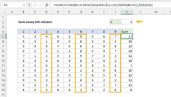
A classic solution to "nth" problems is to use the MOD function to check a numeric array for a remainder of zero after dividing by n. This is the approach in the worksheet shown, there the formula in cell O5, copied down, is:
=MAX(FILTER(B5:M5,MOD(SEQUENCE(,COLUMNS(B5:M5)),n)=0))
At a high level, the FILTER function is configured to retrieve only the nth values of interest using logic created with MOD and SEQUENCE. The result from FILTER is returned to MAX, which returns the maximum value as a final result. Working from the inside out, the SEQUENCE function is configured to generate a numeric array like this:
SEQUENCE(,COLUMNS(B5:M5))
Because there are 12 columns in the range B5:M5, SEQUENCE returns an 1 x 12 array like this:
{1,2,3,4,5,6,7,8,9,10,11,12}
This array is returned to the MOD function as the number argument, with n provided as the divisor. The result from MOD is then compared to zero:
MOD({1,2,3,4,5,6,7,8,9,10,11,12},n)=0
With the number 3 in cell M2 for n, MOD returns an array like this:
{1,2,0,1,2,0,1,2,0,1,2,0}=0
Note that every 3rd value is zero. When this array is compared to zero, the result is an array of TRUE and FALSE values like this:
{FALSE,FALSE,TRUE,FALSE,FALSE,TRUE,FALSE,FALSE,TRUE,FALSE,FALSE,TRUE}
Notice that every 3rd value is now TRUE. This array is returned directly to the FILTER function as the include argument. With array given as B5:M5, FILTER returns every 3rd value in B5:M5 directly to MAX like this:
=MAX({17,1,8,10})
The MAX function then returns 17 as a final result.
CHOOSECOLS + SEQUENCE
An alternative approach is to use the CHOOSECOLS function with the SEQUENCE function like this:
=MAX(CHOOSECOLS(B5:M5,SEQUENCE(,COLUMNS(B5:M5)/n,n,n)))
This formula calculates the numeric indices of target nth values directly, then requests just those values with the CHOOSECOLS function. The SEQUENCE function is configured to return the numeric indexes of every nth value like this:
SEQUENCE(,COLUMNS(B5:M5)/n,n,n)))
The rows argument is left empty. The columns argument is calculated by dividing the number of columns by n. Both start and step are assigned the value n. With 12 columns in B5:M5, and the number 3 for n, this simplifies to:
SEQUENCE(,4,3,3))
The result is a numeric array of "target nth values" like this:
{3,6,9,12}
This array is returned directly to the CHOOSECOLS function as the second argument:
=MAX(CHOOSECOLS(B5:M5,{3,6,9,12}))
The CHOOSECOLS function then returns the values at these locations in an array to MAX:
=MAX({17,1,8,10})
The MAX function returns 17 as before.
All in one formulas
If desired, you can adapt the formulas above to single, all-in-one formulas based on the BYROW function like this:
=BYROW(B5:M16,LAMBDA(r,MAX(FILTER(r,MOD(SEQUENCE(,COLUMNS(r)),n)=0))))
=BYROW(B5:M16,LAMBDA(r,MAX(CHOOSECOLS(r,SEQUENCE(,COLUMNS(r)/n,n,n)))))
The first formula uses the SEQUENCE and MOD approach, the second formula uses the SEQUENCE and CHOOSECOLS approach. Both formulas will return the max values for nth columns for all rows at once.
Legacy Excel
In older versions of Excel without dynamic array formulas like FILTER and SEQUENCE, you can use an array formula like this:
{=MAX(IF(MOD(COLUMN(B5:M5)-COLUMN(B5)+1,n)=0,B5:M5))}
This is an array formula and must be entered with control + shift + enter in older versions of Excel.
At a high level, this formula uses the IF Function together with the MOD and COLUMN functions to "cancel out" values not in nth columns, then runs MAX on the result. The key is this snippet:
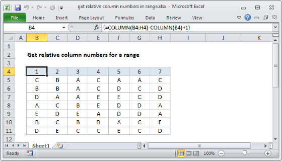
MOD(COLUMN(B5:M5)-COLUMN(B5)+1,n)
The COLUMN function is used to get a set of "relative" column numbers as explained in detail here. The result is a numeric array that starts with the number 1:
{1,2,3,4,5,6,7,8,9,10,11,12}
This array goes into the MOD function as the number argument:
MOD({1,2,3,4,5,6,7,8,9,10,11,12},n)=0
where n is the value to use for "nth". The MOD function returns the remainder for each column number divided by n. When n = 3, MOD will return an array like this:
{1,2,0,1,2,0,1,2,0,1,2,0}
Note that zeros appear for columns 3, 6, 9 and 12, corresponding to every 3rd column. This array is compared to zero with the logical expression =0 to force a TRUE when the remainder is zero and a FALSE when not. These values go into the IF function as the logical test. The IF function then "filters" results so only values in the original range in nth columns make it into the final array. Other values become FALSE. The result is delivered to the MAX function:
=MAX({FALSE,FALSE,17,FALSE,FALSE,1,FALSE,FALSE,8,FALSE,FALSE,10})
The MAX function automatically ignores FALSE values and returns 17 as a final result.
Max of every other column
To get the maximum value in every other column, you can make a small adjustment to the formula when needed. To get the maximum value in even columns, use the original formula with 2 as n:
=MAX(FILTER(data,MOD(SEQUENCE(,COLUMNS(data)),2)=0))
To get the maximum number in odd columns use 2 for n and compare the result to 1:
=MAX(FILTER(data,MOD(SEQUENCE(,COLUMNS(data)),2)=1))
In older versions of Excel, you can use these generic formulas:
{=MAX(IF(MOD(COLUMN(A1:Z1)-COLUMN(A1)+1,2)=0,rng))} // even columns
{=MAX(IF(MOD(COLUMN(A1:Z1)-COLUMN(A1)+1,2)=1,rng))} // odd columns
These are array formulas and must be entered with control + shift + enter in older versions of Excel.