IF with boolean logic

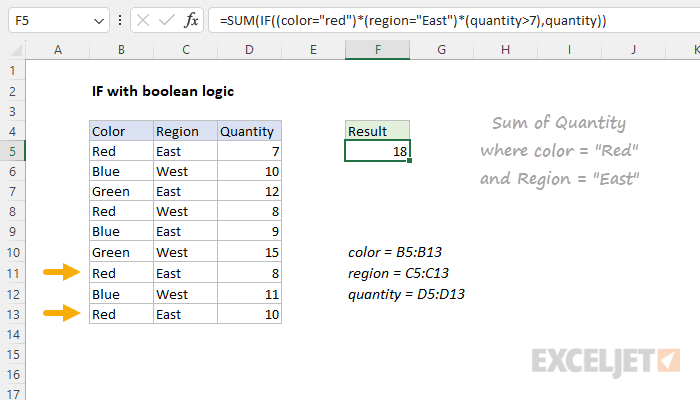
The goal is to sum the quantity for rows where the color is "Red", the region is "East", and the quantity is greater than 7. Although there are a number of ways to solve this problem in Excel purpose of this example is to demonstrate how to replace a nested IF with a single IF using Boolean logic. This technique can be used to reduce the complexity of certain formulas. However, the example is for illustration only. This particular problem could be easily solved with SUMIFS or SUMPRODUCT.

Nested IF approach

One way to solve this problem is by using three separate IF formulas like this:

IF(color="red",IF(region="east",IF(quantity>7,quantity)))

Each IF statement generates an array of TRUE and FALSE values like this:

=IF({TRUE;FALSE;FALSE;TRUE;FALSE;FALSE;TRUE;FALSE;TRUE},
IF({TRUE;FALSE;TRUE;FALSE;TRUE;FALSE;TRUE;FALSE;TRUE},
IF({FALSE;TRUE;TRUE;TRUE;TRUE;TRUE;TRUE;TRUE;TRUE},quantity)))

Only quantities where all three logical tests return TRUE "survive" the operation. Other quantities become FALSE and are evaluated by SUM as zero. The final result inside the SUM function is an array of values like this:

=SUM({FALSE;FALSE;FALSE;FALSE;FALSE;FALSE;8;FALSE;10})

The SUM function ignores the FALSE values and returns 18 as a final result.

Boolean logic approach

Another way to solve this problem is with Boolean logic. In the worksheet shown, we have this formula:

=SUM(IF((color="red")*(region="East")*(quantity>7),quantity))

Notice this formula contains just one IF function. Inside, IF, the logical test is this part:

(color="red")*(region="East")*(quantity>7)

Each expression generates an array of TRUE and FALSE values:

{TRUE;FALSE;FALSE;TRUE;FALSE;FALSE;TRUE;FALSE;TRUE}*{TRUE;FALSE;TRUE;FALSE;TRUE;FALSE;TRUE;FALSE;TRUE}*{FALSE;TRUE;TRUE;TRUE;TRUE;TRUE;TRUE;TRUE;TRUE}

When these arrays are multiplied together, the math operation coerces the TRUE and FALSE values to 1s and 0s. The result is a single array inside the IF function like this:

IF({0;0;0;0;0;0;1;0;1},quantity)

The array of 1s and 0s works to filter out quantities that don't meet all three conditions and the result from IF is the same as we saw above with the nested IF approach:

=SUM({FALSE;FALSE;FALSE;FALSE;FALSE;FALSE;8;FALSE;10})

As before, SUM returns a final result of 18.

Without the IF function

It is possible to remove the IF function altogether and use only Boolean algebra like this:

=SUM((color="red")*(region="East")*(quantity>7)*quantity)

This formula works fine, but it must be entered as an array formula in Excel 2019 and older. To avoid that requirement, you can switch to the SUMPRODUCT function:

=SUMPRODUCT((color="red")*(region="East")*(quantity>7),quantity)
=SUMPRODUCT((color="red")*(region="East")*(quantity>7)*quantity)

Both formulas above return the same result and don't require special handling in older versions of Excel since SUMPRODUCT can handle many array operations natively  For a more detailed example, see SUMPRODUCT with IF

Note: Boolean logic works especially well in formulas that sum values, because non-matching values result in zeros, and zeros do not affect the final sum. However, if the goal is to average values, or get the minimum value based on one or more conditions, the Boolean approach can cause an incorrect result because the 0s may affect the final calculation.