If this AND that OR that

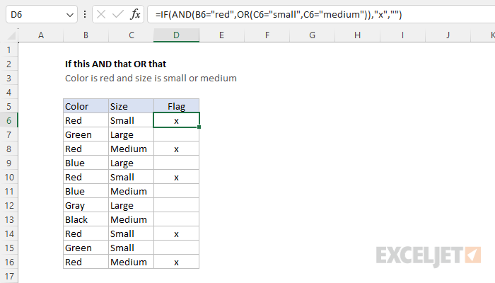
The goal is to mark rows where the color is "Red" AND the size is "Small" or "Medium". To perform this task, you can use the IF function in combination with the AND function and the OR function.

IF function

The IF function runs a test, then returns one value if the result is TRUE, and a different value if the result is FALSE. The generic syntax for IF looks like this:

=IF(logical_test,value_if_true,value_if_false)

For example, if cell A1 contains the value 75, then you could use IF to return "Pass" or "Fail" like this:

=IF(A1>70,"Pass","Fail") // returns "Pass"

If the value in A1 is 65, then the same formula will return "Fail":

=IF(A1>70,"Pass","Fail") // returns "Fail"

Notice that the text values inside IF must be enclosed in double quotes ("").

AND function

The AND function returns TRUE if all conditions are TRUE. For example, if cell A1 contains "Red" and B1 contains 10, then this formula returns TRUE because both expressions return TRUE:

=AND(A1="Red",B1>5) returns TRUE

However, this formula returns FALSE because the second condition returns FALSE:

=AND(A1="Red",B1>12) returns FALSE

Because the AND function returns TRUE or FALSE, it often appears inside the IF function as a logical test, specifying the conditions to be checked.

OR function

The OR function returns TRUE if any condition is TRUE. For example, if cell A1 contains "Red" and B1 contains 10, then this formula returns TRUE because both expressions are TRUE:

=OR(A1="Red",B1>5) returns TRUE

However, if only the first condition is met, the formula will still return TRUE:

=OR(A1="Red",B1>12) returns TRUE

This formula returns FALSE because both conditions are FALSE:

=OR(A1="Blue",B1>12) returns FALSE

AND with OR

The AND function can be combined with the OR function. In the example shown, we want to identify records where the color is Red and the size is Small or Medium. This means we need to test the value in column B for "Red" and test the value in column C for "Small" or "Medium". We can do that by nesting the OR function inside the AND function like this:

AND(B6="red",OR(C6="small",C6="medium"))

Note: Excel formulas are not case-sensitive by default, so B6="red", B6="Red", and B6="RED" will all return the same result. For that reason, the text values in the logical test are left in lowercase.

The formula above will return TRUE only if the value in B6 is "Red" AND the value in C6 is "Small" OR "Medium". In any other case, the formula will return FALSE. The formula evaluates the side function first, working outwards. The OR function returns a result to AND, and the AND function returns the final result. This is exactly what we need for the logical test inside IF.

Final formula

To process the result from AND and mark a row with an "x" when both conditions are TRUE, we embed the AND formula inside the IF function as the logical test. In D6, the formula is:

=IF(AND(B6="red",OR(C6="small",C6="medium")),"x","")

If the result from AND is TRUE, the IF function returns "x". If the result is FALSE, the IF function returns an empty string (""), which looks like an empty cell in Excel. As the formula is copied down column D, the result is an "x" in column D only when the color is Red and the size is Small or Medium. The result from IF can be customized as needed.

Note: You might wonder if we need to supply an empty string ("") for the false result. Technically, this argument is optional. However, without a value, the IF function will return and display FALSE for rows that don't meet the specified conditions.