Summary
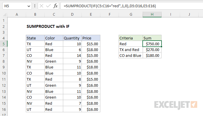
To create a conditional sum with the SUMPRODUCT function you can use the IF function or use Boolean logic. In the example shown, the formula in H5 is:
=SUMPRODUCT(IF(C5:C16="red",1,0),D5:D16,E5:E16)
The result is $750, the total value of items with a color of "Red" in the data as shown. Note that SUMPRODUCT is not case-sensitive. Using the IF function inside SUMPRODUCT makes this into an array formula that must be entered with control + shift + enter in Legacy Excel. See below for an alternative Boolean syntax that does not need special handling.
Generic formula
=SUMPRODUCT(IF(criteria,1,0),values)
Explanation
In this example, the goal is to calculate a conditional sum with the SUMPRODUCT function to match the criteria shown in G5:G7. One way to do this is to use the IF function directly inside of SUMPRODUCT. Another more common alternative is to use Boolean logic to apply criteria. Both approaches are explained below.
Basic SUMPRODUCT
The SUMPRODUCT function multiplies ranges or arrays together and returns the sum of products. The classic SUMPRODUCT problem multiplies two ranges together and sums the product directly without a helper column. For example, in the worksheet above, we have Quantity and Price, but no line item total. You can use SUMPRODUCT to get the total value of all records in the data like this:
=SUMPRODUCT(D5:D16,E5:E16)
In the worksheet shown, the result is $1,882, the sum of all quantities in D5:D16 multiplied by all prices in E5:E16. This formula works nicely. However, it's not obvious how to calculate a conditional sum with SUMPRODUCT. For example, how can you calculate the value of all records where the color is "Red"? One option is to use the IF function directly, as explained in the next section.
SUMPRODUCT + IF function
One way to apply conditions with the SUMPRODUCT function is to use the IF function directly. This is the approach seen in the worksheet shown, where the formula in cell H5 is:
=SUMPRODUCT(IF(C5:C16="red",1,0),D5:D16,E5:E16)
In this configuration, SUMPRODUCT has been given three arguments, array1, array2, and array3. Note that array2 holds Quantity and array3 holds Price. It is array1 that applies the conditional logic with the IF function like this:
IF(C5:C16="red",1,0)
Notice we are using 1 and 0 for the value_if_true and value_if_false arguments instead of the default TRUE and FALSE values. We do this because we want a numeric result, for reasons that become clear below. Because there are 12 values in the range C5:C16, IF returns an array with 12 results like this:
{1;0;1;0;0;0;1;0;0;0;1;1}
In this array, 1s indicate records where the color is "Red" and 0s indicate other colors. Dropping this array back into the SUMPRODUCT function, we have:
=SUMPRODUCT({1;0;1;0;0;0;1;0;0;0;1;1},D5:D16,E5:E16)
Now you can see how the logic works. The Boolean values that make up array1 act like a filter when the arrays are multiplied together. After multiplication, there is just a single array like this:
=SUMPRODUCT({150;0;210;0;0;0;120;0;0;0;126;144})
Note that the value of records where the color is not "Red" have been "zeroed out". The final result returned by SUMPRODUCT is $750. Additional conditions can be added with additional IF statements. To calculate a total for Color = "Red" and State = "TX", you can use the IF function twice like this:
=SUMPRODUCT(IF(C5:C16="red",1,0),IF(B5:B16="tx",1,0),D5:D16,E5:E16)
The result is $270, as you can see in cell H6. The formula in cell H7 calculates a total for color = "Blue" and State = "CO" like this:
=SUMPRODUCT(IF(C5:C16="blue",1,0),IF(B5:B16="co",1,0),D5:D16,E5:E16)
Although this formula works fine, one consequence of using the IF function inside of SUMPRODUCT is that it makes this into an array formula that must be entered with control + shift + enter in older versions of Excel that do not support dynamic array formulas. This is a bit unexpected, because one of SUMPRODUCT's key strengths is the ability to handle array operations natively, but the IF function defeats this feature. The traditional solution to this problem is to switch to Boolean logic, as explained below.
SUMPRODUCT + Boolean logic
An alternative to using the IF function directly inside of SUMPRODUCT is to use Boolean logic. For example, to calculate the total value of records where the color is "Red", you can use a formula like this:
=SUMPRODUCT(--(C5:C16="red"),D5:D16,E5:E16)
This example illustrates one of the key strengths of the SUMPRODUCT function – the ability to handle array operations natively. Inside SUMPRODUCT, the first array is a logical expression to filter on the color "red":
--(C5:C16="red")
SUMPRODUCT is not case-sensitive, so "red" will match "red", "Red", and "RED". Because there are 12 values in the range C5:C16, this expression returns an array with 12 results like this:
--({TRUE;FALSE;TRUE;FALSE;FALSE;FALSE;TRUE;FALSE;FALSE;FALSE;TRUE;TRUE})
The double negative (--) then converts the TRUE and FALSE values to 1s and zeros:
{1;0;1;0;0;0;1;0;0;0}
Back in SUMPRODUCT, we now have:
=SUMPRODUCT({1;0;1;0;0;0;1;0;0;0;1;1},D5:D16,E5:E16)
Notice this is the same result we had with the IF function example above. As before, array1 acts like a filter when the arrays are multiplied together. After multiplication, there is just a single array like this:
=SUMPRODUCT({150;0;210;0;0;0;120;0;0;0;126;144})
All values associated with colors that are not "Red" have been "zeroed out", and the final result is $750. As with the IF function, the same pattern can be repeated to add more conditions. To calculate a total for Color = "Red" and State = "TX", you can use a formula like this:
=SUMPRODUCT(--(B5:B16="tx"),--(C5:C16="red"),D5:D16,E5:E16)
To calculate a total for color = "Blue" and State = "CO", the formula is:
=SUMPRODUCT(--(B5:B16="co"),--(C5:C16="blue"),D5:D16,E5:E16)
Simplifying with a single array
Excel pros will often simplify the syntax inside SUMPRODUCT by placing the conditional logic into a single argument like this
=SUMPRODUCT((B5:B16="co")*(C5:C16="blue"),D5:D16,E5:E16)
One advantage of this approach is that the math operation in array1 automatically coerces TRUE and FALSE into 1s and 0s, so we don't need a double negative (--). Another advantage is that the math operation can be changed to apply a different type of logic. Instead of multiplication (*), which corresponds to AND logic in Boolean algebra, you can use addition (+), which corresponds to OR logic. For example, to sum the value of all records that are either "Red" or "Blue", you could use a formula like this:
=SUMPRODUCT((C5:C16="red")+(C5:C16="blue"),D5:D16,E5:E16)
As you can see, using Boolean logic with SUMPRODUCT is a flexible alternative to using the IF function, and it offers a major advantage: the formula will work fine in Legacy Excel, with no need to enter as an array formula with control + shift + enter.