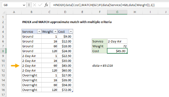
XLOOKUP approximate match with multiple criteria

In this example, we have shipping rate data in the range B5:D16, and the goal is to use XLOOKUP to find the correct shipping cost for an item based on two criteria: (1) the selected service in G6 (exact match) and (2) the weight in G7 (approximate match). The screen below shows the basic idea:

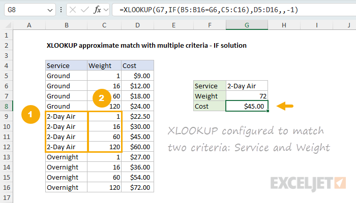
The exact match is straightforward: If a user enters "2-Day Air" in cell G6, we want to match that service exactly in the lookup table and ignore other rows. The second condition involves looking up the weight entered in cell G7 and finding the "correct" match. Most likely, we will not find an exact match, so we will need to scan through the entries until we find a larger weight value and then drop back to the previous row. This is the meaning of an "approximate match" in this example, and it is what makes the problem challenging. The approximate match requirement means we cannot use a simpler formula based on Boolean logic, which requires an exact match.

The article below shows how to solve this problem in two different ways. In the first approach, we use XLOOKUP + the IF function to apply criteria. In the second approach, we use the XLOOKUP with the FILTER function, which requires a bit more configuration. Both formulas are explained in detail below.

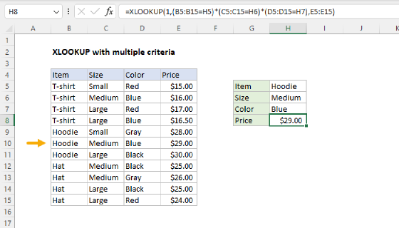
If you need an exact match with multiple criteria, see XLOOKUP with multiple criteria.

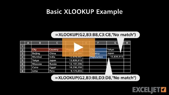
If you are new to XLOOKUP, this short video shows a basic example.

Table of contents

• Basic XLOOKUP approximate match
• XLOOKUP with Boolean logic
• XLOOKUP with IF
• XLOOKUP with FILTER
• Summary

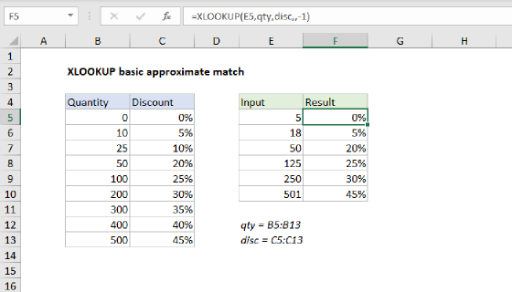
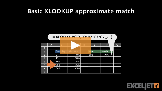
Basic XLOOKUP approximate match

Before we get into the details of the formulas below, let's review how to perform a basic approximate match with XLOOKUP. The worksheet below shows a simplified example of the problem above with the Service removed. The goal is to look up the weight entered in cell F4 and return the appropriate cost in cell F5. Because we are unlikely to find an exact match on the weight, we need to perform an approximate match. XLOOKUP should scan through the values in B5:B8, looking for the weight in F4. If it finds an exact match, it should stop and return the cost on that row. If it finds a value greater than F4 (which means an exact match was not found), it should drop back to the previous row and return the cost from that row. The formula in cell F5 looks like this:

=XLOOKUP(F4,B5:B8,C5:C8,,-1)

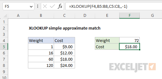
The lookup_array is the weight in the range B5:B8, and the return_array is the cost in the range C5:C8. Notice the match_mode argument inside XLOOKUP is set to -1, to find the largest value in B5:B8 that is less than or equal to the lookup value in cell F4. In this case, the largest value less than or equal to 72 is 60, so XLOOKUP matches the 60 and returns $18.00 as a final result:

=XLOOKUP(F4,B5:B8,C5:C8,,-1) // returns 18

We now have a simple working XLOOKUP formula that returns the correct cost based on an approximate match lookup. The challenge is that we also need to match based on the Service. To do that, we need to extend the formula to handle another condition. Let's look first at why we can't use Boolean logic like we can in simple exact match scenarios.

XLOOKUP with Boolean logic

Before we get to the working solutions explained below, let's take a quick look at why we can't use Boolean logic in this case. Boolean logic involves running logical tests that return TRUE and FALSE and using simple math operations that coerce the TRUE/FALSE values to 1s and 0s. You can use Boolean logic inside the XLOOKUP function to evaluate multiple criteria. For example, to evaluate two criteria, the generic formula would look like this:

=XLOOKUP(1,(range=A1)*(range=B1),return_array)

The key idea is that the expression (range=A1)*(range=B1) will return an array of 1s and 0s, and XLOOKUP is configured to look for a 1. For example, if the range contains 12 rows and the third row matches both conditions, the formula will evaluate like this:

=XLOOKUP(1,{0,0,1,0,0,0,0,0,0,0,0,0},return_array)

Then, XLOOKUP will return the third value in return_array as the final result. For a detailed explanation of this concept with an example, see XLOOKUP with multiple criteria.

This works great if all criteria require exact matches. However, if we try to adapt this formula to handle the problem in the example, which requires an approximate match, we might try something like this:

=XLOOKUP(1,(B5:B16=G6)*(C5:C16<=G7),D5:D16)

However, this fails, as you can see in the workbook below:

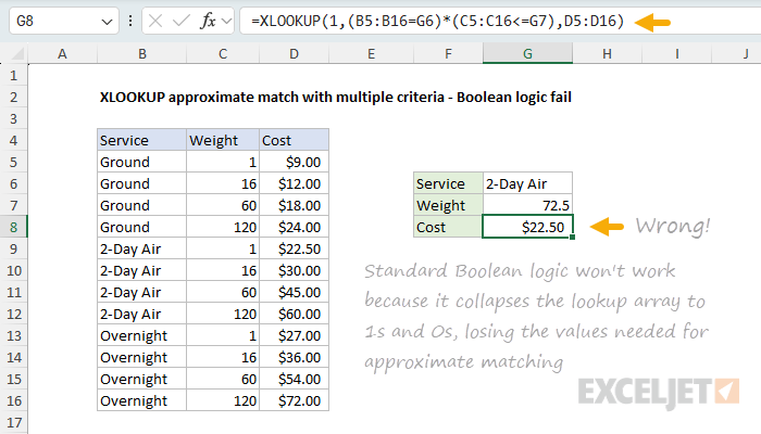
The reason it fails is that converting the lookup_array to 1s and 0s removes the values required for approximate matching. You can see this happen when we trace the evaluation of the formula:

=XLOOKUP(1,(B5:B16=G6)*(C5:C16<=G7),D5:D16)
=XLOOKUP(1,{0;0;0;0;1;1;1;0;0;0;0;0},D5:D16)
=22.5

Notice the lookup_array ends up containing only 1s and 0s. When XLOOKUP runs, it matches the first 1 found, returning an incorrect result from D5:D16. In the next section, we'll look at a different way to apply multiple criteria that leaves the values needed for approximate matching intact.

I should note that it it is possible to make the XLOOKUP formula above work by providing a -1 for search_mode. However, I think this is confusing. Match mode -1 means "find the largest value that doesn't exceed the lookup value," and search mode -1 means "search from last to first." They perform different jobs, and using search mode like this mixes things together in a way that is conceptually hard to untangle and explain. In addition, since there are multiple 1s in the mix, the data must be sorted in a particular way, which is not the case with the IF and FILTER approaches.

XLOOKUP with IF

As shown above, we know how to set-up XLOOKUP to perform an approximate match based on weight. The remaining challenge is that we also need to take into account the Service. One approach is to "filter out" extraneous entries in the table so we are left only with entries that correspond to the Service we are looking up, and the classic way to do this is with the IF function. This is the approach used in the worksheet shown, where the formula in cell G8 is:

=XLOOKUP(G7,IF(B5:B16=G6,C5:C16),D5:D16,,-1)

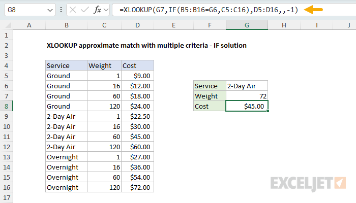
The filtering is done with the IF function, which appears inside the XLOOKUP function like this:

IF(B5:B16=G6,C5:C16)

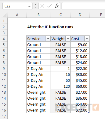
This code tests the values in the Service column (B) to see if they match the value in G6. Where there is a match, the corresponding values in the Weight column (C) are returned. If there is no match, the IF function returns FALSE. Because there are 12 rows in the table, the IF function returns an array that contains 12 results like this:

{FALSE;FALSE;FALSE;FALSE;1;16;60;120;FALSE;FALSE;FALSE;FALSE}

Notice the only weights that remain in the array are those that correspond to the "2-Day-Air" service; all other weights have been replaced with FALSE. You can visualize this operation in the original data as shown below:

This array is delivered directly to XLOOKUP as the lookup_array:

=XLOOKUP(G7,{FALSE;FALSE;FALSE;FALSE;1;16;60;120;FALSE;FALSE;FALSE;FALSE},D5:D16,,-1)

With a weight of 72 in cell G7, XLOOKUP matches 60 and returns $45.00 as the final result. Notice that we are using -1 inside XLOOKUP as the match_mode argument. This will cause XLOOKUP to find the largest value that doesn't exceed the lookup value.

One reason this works nicely is that the IF function returns 12 results, which correspond to the 12 rows in the table. This means XLOOKUP can simply return the corresponding weight from D5:D16 because all 12 rows are still intact.

XLOOKUP with FILTER

Another way to solve this problem is with XLOOKUP and the FILTER function. You can see an example of this approach in the worksheet below, where the formula in G8 is:

=XLOOKUP(G7,FILTER(C5:C16,B5:B16=G6),FILTER(D5:D16,B5:B16=G6),,-1)

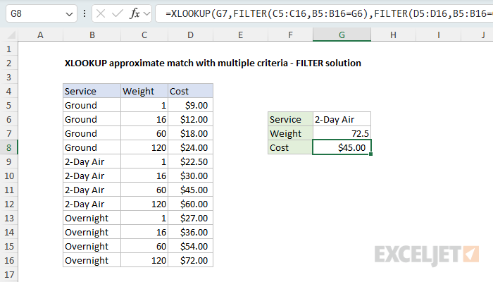
In this formula, we remove data for other services with the FILTER function. Inside XLOOKUP, FILTER creates the lookup_array like this:

FILTER(C5:C16,B5:B16=G6) // returns {1;16;60;120}

The return_array is created in the same way:

FILTER(D5:D16,B5:B16=G6) // returns {22.5;30;45;60}

After FILTER runs, XLOOKUP is only working with values associated with the 2-Day air service:

=XLOOKUP(G7,{1;16;60;120},{22.5;30;45;60},,-1)

With 72 in cell G7, XLOOKUP returns the same result as before, a cost of $45.00. This formula works nicely and is perhaps more intuitive than XLOOKUP + IF. However, the tradeoff is a bit more complexity since FILTER must be used twice, once for the lookup array and once for the return array. You can tidy up the formula a bit by adding the LET function and creating a "match" array like this:

=LET(
    match,B5:B16=G6,
    XLOOKUP(G7,FILTER(C5:C16,match), FILTER(D5:D16,match),, -1)
)

This saves the Boolean array created by B5:B16=G6 so that it's only evaluated once and reused in both FILTER calls. We still need to call FILTER twice (one for the lookup array, one for the return array), but both calls use the same saved criteria, which makes the formula more efficient and easier to read.

Summary

To perform an approximate match lookup with multiple criteria in XLOOKUP, the key challenge is that standard Boolean logic won't work because it collapses the lookup array to 1s and 0s, losing the values needed for approximate matching. Two effective approaches are: (1) use the IF function inside XLOOKUP to replace non-matching entries with FALSE while preserving the actual lookup values, or (2) use the FILTER function to remove non-matching rows entirely from both the lookup and return arrays. The IF approach is simpler and more compact, while the FILTER approach is more intuitive but requires filtering both arrays. Adding LET to the FILTER approach can improve readability by saving the criteria expression for reuse.