Summary
To lookup information associated with the lowest value in table, you can use a formula based on INDEX, MATCH, and MIN functions.
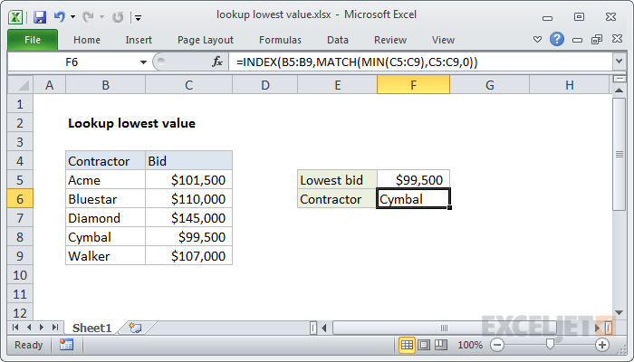
In the example shown, a formula is used to identify the name of the contractor with the lowest bid. The formula in F6 is:
=INDEX(B5:B9,MATCH(MIN(C5:C9),C5:C9,0))
Generic formula
=INDEX(range,MATCH(MIN(vals),vals,0))
Explanation
Working from the inside out, the MIN function is used to find the lowest bid in the range C5:C9:
MIN(C5:C9) // returns 99500
The result, 99500, is fed into the MATCH function as the lookup value:
MATCH(99500,C5:C9,0) // returns 4
Match then returns the location of this value in the range, 4, which goes into INDEX as the row number along with B5:B9 as the array:
=INDEX(B5:B9, 4) // returns Cymbal
The INDEX function then returns the value at that position: Cymbal.