Summary
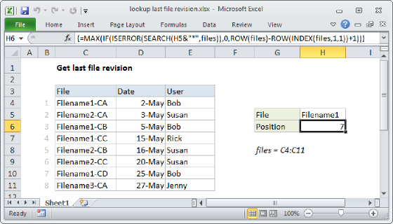
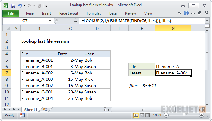
To lookup the latest file version in a list, you can use a formula based on the LOOKUP function together with the ISNUMBER and FIND functions. In the example shown, the formula in cell G7 is:
=LOOKUP(2,1/(ISNUMBER(FIND(G6,files))),files)
where "files" is the named range B5:B11.
Context
In this example, we have a number of file versions listed in a table with a date and user name. Note that file names are repeated with a counter at the end as a revision number - 001, 002, 003, etc.
Given a file name, we want to retrieve the name of the last or latest revision. There are two challenges:
- The challenge is the version codes at the end of the file names make it harder to match the file name.
- By default, Excel match formulas will return the first match, not the last match.
To overcome these challenges, we need to use some tricky techniques.
Generic formula
=LOOKUP(2,1/(ISNUMBER(FIND(filename,range))),range)
Explanation
This formula uses the LOOKUP function to find and retrieve the last matching file name. The lookup value is 2, and the lookup_vector is created with this:
1/(ISNUMBER(FIND(G6,files)))
Inside this snippet, the FIND function looks for the value in G6 inside the named range "files" (B5:B11). The result is an array like this:
{1;#VALUE!;1;1;#VALUE!;#VALUE!;1}
Here, the number 1 represents a match, and the #VALUE error represents a non-matching file name. This array goes into the ISNUMBER function and comes out like this:
{TRUE;FALSE;TRUE;TRUE;FALSE;FALSE;TRUE}
Error values are now FALSE, and the number 1 is now TRUE. This overcomes challenge #1, we now have an array that shows clearly which files in the list contain the file name of interest.
Next, the array is used as the denominator with 1 as numerator. The result looks like this:
{1;#DIV/0!;1;1;#DIV/0!;#DIV/0!;1}
which goes into LOOKUP as the lookup_vector. This is a tricky solution to challenge #2. The LOOKUP function operates in approximate match mode only, and automatically ignores error values. This means with 2 as a lookup value, VLOOKUP will try to find 2, fail, and step back to the previous number (in this case matching the last 1 in position 7). Finally, LOOKUP uses 7 like an index to retrieve the 7th file in the list of files.
Handling blank lookups
Oddly, the FIND function returns 1 if the lookup value is an empty string (""). To guard against a false match, you can wrap the formula in IF and test for an empty lookup:
=IF(G6<>"",LOOKUP(2,1/(ISNUMBER(FIND(G6,files))),files),"")