Summary
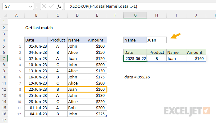
To get the last match in a set of data you can use the XLOOKUP function. In the example shown, the formula in G7 is:
=XLOOKUP(H4,data[Name],data,,,-1)
Where data is an Excel Table in the range B5:B16. The result, in this case, is the last entry for 'Juan', which is row 8 in the table.
Generic formula
=XLOOKUP(A1,range,range,,,-1)
Explanation
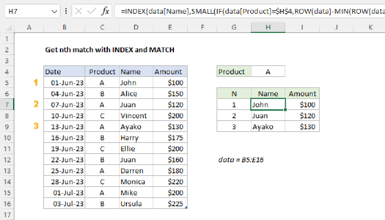
In the example shown, we have a set of order data that includes Date, Product, Name, and Amount. The data is sorted by date in ascending order. The goal is to look up the latest order for a given person by Name. In other words, we want the last match by name. The challenge is that Excel lookup formulas will return the first match by default. There are several ways to approach this problem. In the current version of Excel, a good option is the XLOOKUP function. Another more flexible approach is to use the FILTER function with the TAKE function. In an older version of Excel, the easiest approach is to use a formula based on the LOOKUP function. All three approaches are explained below.
XLOOKUP function
One way to solve this problem is with the XLOOKUP function, which is a modern upgrade to the VLOOKUP function. XLOOKUP is a very flexible function that takes six separate arguments:
=XLOOKUP(lookup,lookup_array,return_array,[if_not_found],[match_mode],[search_mode])
Where each input has the following meaning:
- lookup_value - the value to look for
- lookup_array - the range or array to search within
- return_array - the range or array to return values from
- if_not_found - value to return if no match is found
- match_mode - settings for exact, approximate, and wildcard matching
- search_mode - settings for first, last, and binary searches
To solve this problem with XLOOKUP, you only need four of the parameters listed above:
=XLOOKUP(lookup,lookup_array,return_array,,,search_mode)
The key input is search_mode, which is needed to enable a reverse search. In the worksheet shown, the formula in cell G7 is:
=XLOOKUP(H4,data[Name],data,,,-1)
The inputs to XLOOKUP are:
- lookup_value: H4 (search value)
- lookup_array: data[Name]
- return_array: data (the entire table)
- search_mode: -1 for search last-to-first
The last input, search_mode, is provided as -1 to create the last match behavior. In this configuration, XLOOKUP looks for the name "Juan" in the Name column of the table, starting from the bottom. When it finds a match, it returns the entire matching row from the data table. Notice we leave if_not_found and match_mode empty, but we still need to supply the commas. Feel free to supply any value you like for if_not_found. Match_mode is not necessary, because XLOOKUP operates in exact-match mode by default, which is what we want in this case. It is not necessary to return the entire row. To return just the amount, simply adjust return_array, as needed. For example, to return just Amount, use data[Amount] like this:
=XLOOKUP(H4,data[Name],data[Amount],,,-1) // amount only
For more details on XLOOKUP, see How to use the XLOOKUP function. Excel Tables use structured references like data[Name]. See Excel Tables for a complete overview.
Last n matches
Another way to solve this problem is to use the FILTER function with the TAKE function like this:
=TAKE(FILTER(data,data[Name]=H4),-1)
Essentially, we are filtering the entire set of data by name, then grabbing the last record from the filtered data with TAKE. This is a more flexible approach because it can be used to get the "last n matches". The generic version of the formula looks like this:
=TAKE(FILTER(range,logical_test),-n)
For example, to get the last two matches in the worksheet shown, you can use:
=TAKE(FILTER(data,data[Name]=H4),-2)
Here, the FILTER function is configured to return all matching records by name using the value in H4, and the TAKE function is configured to return the last two records returned by FILTER, starting from the bottom, by providing -2 for the rows argument.
Note: For more details on FILTER and TAKE, see How to use the FILTER function and How to use the TAKE function.
nth to last match
If you want the nth to last match (i.e. the second to the last match, the third to the last match, etc.) you can replace TAKE with the CHOOSEROWS function like this:
=CHOOSEROWS(FILTER(data,data[Name]=H4),-n)
Where n represents the number of the match you want. For example, to get the second to last match, you can use:
=CHOOSEROWS(FILTER(data,data[Name]=H4),-2)
FILTER returns all matching rows as before. CHOOSEROWS then returns the second to last row from the FILTER result. Keep in mind that there may not be a second-to-last match and, in that case, CHOOSEROWS will return a #VALUE! error.
XMATCH function
The example shown returns the data from the location of the last match. If you only want the location of the last match, you can use the XMATCH function like this:
=XMATCH(H4,data[Name],,-1) // returns 8
As with XLOOKUP, the search_mode argument is set to -1 to enable last-to-first matching. The result is 8 since the last match is in the eighth row of the table. To retrieve the matching row, nest the XMATCH formula above inside the INDEX function like this:
=INDEX(data,XMATCH(H4,data[Name],,-1),0)
Note that row_num must be provided as zero to return an entire row with INDEX. For more details, see:
Older versions of Excel
In older versions of Excel that do not provide XLOOKUP or XMATCH, you can use a formula based on the LOOKUP function. LOOKUP is an older function in Excel that can work well in "last match" scenarios, because it can handle array operations in older versions of Excel natively, with no need to enter as an array formula with control + shift + enter. In this problem, we can use LOOKUP in a formula like this:
=LOOKUP(2,1/(data[Name]=H4),data[Amount])
This formula finds the last Amount for Juan in the data, which is 160. Let's look at how this works step by step. Working from the inside out, we first apply the criteria with a simple logical expression:
data[Name]=H4
With "Juan" in cell H4, this expression results in an array of 12 TRUE and FALSE values, where TRUE corresponds to names equal to "Juan" in the Name column:
{FALSE;FALSE;TRUE;FALSE;FALSE;FALSE;FALSE;TRUE;FALSE;FALSE;FALSE;FALSE}
Notice, we have TRUE values at rows 3 and 8. Next, we divide the number 1 by this array. During division, the math operation coerces TRUE to 1 and FALSE to zero, so you should visualize the operation like this:
1/{0;0;1;0;0;0;0;1;0;0;0;0}
When the actual division takes place, one divided by one is one, and one divided by zero creates a #DIV/0 error and the resulting array looks like this:
{#DIV/0!;#DIV/0!;1;#DIV/0!;#DIV/0!;#DIV/0!;#DIV/0!;1;#DIV/0!;#DIV/0!;#DIV/0!;#DIV/0!}
This array is the lookup_vector inside LOOKUP, so at this point, we have:
=LOOKUP(2,{#DIV/0!;#DIV/0!;1;#DIV/0!;#DIV/0!;#DIV/0!;#DIV/0!;1;#DIV/0!;#DIV/0!;#DIV/0!;#DIV/0!},data[Amount])
Notice that the lookup value is 2. This may seem strange, but it is intentional. We use 2 as a lookup value to force LOOKUP to scan to the end of the data. LOOKUP will automatically ignore errors, so the only thing left to match are the 1s. It will scan through the 1s looking for a 2 that can never be found. When it reaches the end of the array, it will "step back" to the last valid value (the last 1), and return the Amount from the row at that position.
Row numbers and nth last match
The workarounds needed in older versions of Excel can be very complex. This section is quite technical and not necessary unless you want to use INDEX and MATCH to get the last match in an older version of Excel. Personally, I would try the LOOKUP alternative above first and only use the approach described below if there is a reason LOOKUP does not work as required. Nonetheless, it is useful to see how these things can be done in older versions of Excel and it provides a nice contrast to the simplicity of the XLOOKUP and FILTER + TAKE options explained above.
Note: The formulas in this section are array formulas and must be entered with control + shift + enter in Excel 2019 and older.
Getting the row number (and ultimately, the value) for the nth last match is more difficult in older versions of Excel because we have no direct way to perform a reverse search. One option to get "nth last row numbers" is to use an array formula like this:
=LARGE(IF(criteria,ROW(rng)-MIN(ROW(rng))+1),k)
where k represents "nth", as seen below:
=LARGE(IF(data[Name]=H4,ROW(data)-MIN(ROW(data))+1),1) // last match
=LARGE(IF(data[Name]=H4,ROW(data)-MIN(ROW(data))+1),2) // 2nd last
=LARGE(IF(data[Name]=H4,ROW(data)-MIN(ROW(data))+1),3) // 3rd last
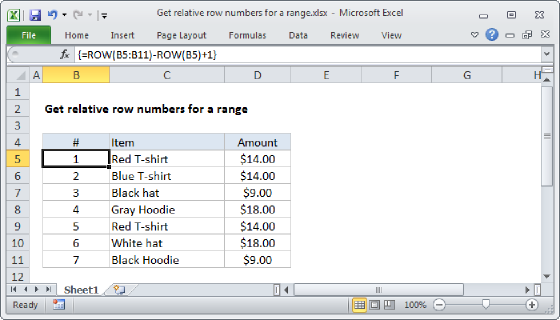
Working from the inside out, this part of the formula will generate a relative set of row numbers:
ROW(data)-MIN(ROW(data))+1
The result of the above expression is an array of numbers like this:
{1;2;3;4;5;6;7;8;9;10;11;12}
Notice we get 12 numbers, corresponding to the 12 rows in the table. Next, we only want row numbers for matching values, so we use the IF function to filter the values like so:
IF(data[Name]=H4,ROW(data)-MIN(ROW(data))+1)
This results in an array like this:
{FALSE;FALSE;3;FALSE;FALSE;FALSE;FALSE;8;FALSE;FALSE;FALSE;FALSE}
Note this array still contains 12 values, but only the row numbers where the name equals H4 ("Juan") survive. All other values become FALSE since they failed the logical test in the IF function. Finally, the array is delivered to the LARGE function, which extracts the nth largest value, which corresponds to the nth last match:
LARGE({FALSE;FALSE;3;FALSE;FALSE;FALSE;FALSE;8;FALSE;FALSE;FALSE;FALSE},1) // returns 8
LARGE({FALSE;FALSE;3;FALSE;FALSE;FALSE;FALSE;8;FALSE;FALSE;FALSE;FALSE},2) // returns 3
Once we know the last matching row number, we can use INDEX to retrieve a value at that position. The final formula looks like this:
=INDEX(data[Amount],LARGE(IF(data[Name]=H4,ROW(data)-MIN(ROW(data))+1),n))
With "Juan" in cell H4, we get the following:
=INDEX(data[Amount],LARGE(IF(data[Name]=H4,ROW(data)-MIN(ROW(data))+1),1)) // 160
=INDEX(data[Amount],LARGE(IF(data[Name]=H4,ROW(data)-MIN(ROW(data))+1),2)) // 120
For more details on INDEX with MATCH, see How to use INDEX and MATCH.