Summary
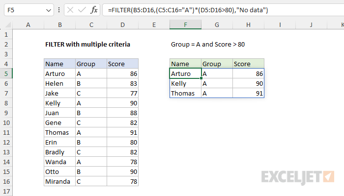
To filter data with multiple criteria, you can use the FILTER function and simple boolean logic expressions. In the example shown, the formula in F5 is:
=FILTER(B5:D16,(C5:C16="A")*(D5:D16>80),"No data")
The result returned by FILTER includes only rows where the group is "A" and the score is greater than 80. If no data meets criteria, FILTER returns "No data".
Generic formula
=FILTER(range,(criteria1)*(criteria2),"No data")
Explanation
In this example, the goal is to filter data based on multiple criteria with the FILTER function. Specifically, we want to select data where (1) the group = "A" and (2) the Score is greater than 80. At first glance, it's not obvious how to do this with the FILTER function. Unlike older functions like COUNTIFS or SUMIFS, which provide multiple arguments for entering multiple conditions, the FILTER function only provides a single argument called "include" to filter data. The trick is to create logical expressions that use Boolean algebra to target the data of interest and supply these expressions as the include argument.
FILTER function
The FILTER function "filters" a range of data based on supplied criteria and extracts matching records. The generic syntax for FILTER looks like this:
FILTER(array,include,[if_empty])
The idea with FILTER is that the include argument is provided as a logical expression that targets data of interest. Most of the challenge in using FILTER is developing a logical expression that correctly targets data that meets all conditions.
FILTER with multiple criteria
In this problem, we need to configure FILTER to apply two criteria: (1) Group is "A" and (2) Score is greater than 80. To start off, we provide all data (B5:D16) for the array argument, because we want FILTER to return all three columns:
=FILTER(B5:D16,
Next, we need to supply the logic needed to target records where the Group is "A". We do this with a simple logical expression:
=C5:C16="A"
Here, we compare every value in the Group column to "A". Because we have 12 rows of data, the result is an array that contains 12 TRUE and FALSE values like this:
{TRUE;FALSE;FALSE;TRUE;FALSE;FALSE;TRUE;FALSE;FALSE;TRUE;FALSE;FALSE}
Notice the TRUE values in the array correspond to rows where the Group is "A". If we were to use this expression by itself as the include argument, FILTER will return all 4 rows where the Group is "A". Next, we need to add logic to target records with the second condition: Score is greater than 80. This can be done with another simple logical expression:
=D5:D16>80
Like the previous expression, this snippet will return an array that contains 12 TRUE and FALSE values:
{TRUE;TRUE;FALSE;TRUE;TRUE;TRUE;TRUE;FALSE;TRUE;FALSE;TRUE;FALSE}
In this array, TRUE values indicate rows where the score is greater than 80. At this point, we have two simple logical expressions, and we need to join them inside the include argument. To do this, we need to add parentheses around both expressions (to control the order of operations) and then multiply to two expressions together:
=(C5:C16="A")*(D5:D16>80)
We use multiplication (*) because, under the rules of Boolean algebra, multiplication corresponds to AND logic, and addition (+) corresponds to OR logic.
After each expression is evaluated, we have the following two arrays:
={TRUE;FALSE;FALSE;TRUE;FALSE;FALSE;TRUE;FALSE;FALSE;TRUE;FALSE;FALSE}*{TRUE;TRUE;FALSE;TRUE;TRUE;TRUE;TRUE;FALSE;TRUE;FALSE;TRUE;FALSE}
The math operation of multiplication converts the TRUE and FALSE values to 1s and 0s:
={1;0;0;1;0;0;1;0;0;1;0;0}*{1;1;0;1;1;1;1;0;1;0;1;0}
After multiplication, we have a single array:
={1;0;0;1;0;0;1;0;0;0;0;0}
Notice that the 1s in this array correspond to rows in the data where the Group is "A" and the score is greater than 80. This is exactly what we need to retrieve data that matches both conditions. This array is returned directly to FILTER as the include argument:
=FILTER(B5:D16,{1;0;0;1;0;0;1;0;0;0;0;0},"No data")
The final result from FILTER is the three rows in the data that meet the criteria.