Summary
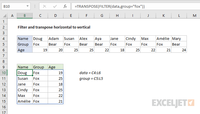
To filter data arranged horizontally and display the result in a vertical format, you can use the FILTER function together with TRANSPOSE. In the example shown, the formula in B10 is:
=TRANSPOSE(FILTER(data,group="fox"))
where data (C4:L6) and group (C5:L5) are named ranges.
Generic formula
=TRANSPOSE(FILTER(data,logic))
Explanation
The goal is to filter the horizontal data in the range C4:L6 to extract members of the group "fox" and display results with data transposed to a vertical format. For convenience and readability, we have two named ranges to work with: data (C4:L6) and group (C5:L5).
The FILTER function can be used to extract data arranged vertically (in rows) or horizontally (in columns). FILTER will return the matching data in the same orientation. The formula in B5 is:
=TRANSPOSE(FILTER(data,group="fox"))
Working from the inside out, the include argument for FILTER is a logical expression:
group="fox" // test for "fox"
When the logical expression is evaluated, it returns an array of 10 TRUE and FALSE values:
{TRUE,FALSE,TRUE,FALSE,FALSE,TRUE,TRUE,TRUE,TRUE,FALSE}
Note: the commas (,) in this array indicate columns. Semicolons (;) would indicate rows.
The array contains one value per record in the data, and each TRUE corresponds to a column where the group is "fox". This array is returned directly to FILTER as the include argument, where it does the actual filtering:
FILTER(data,{TRUE,FALSE,TRUE,FALSE,FALSE,TRUE,TRUE,TRUE,TRUE,FALSE})
Only data in columns that correspond to TRUE make it through the filter, so the result is data for the six people in the "fox" group. FILTER returns this data in the original horizontal structure. Because we want to display results from FILTER in a vertical format, the TRANSPOSE function is wrapped around the FILTER function:
=TRANSPOSE(FILTER(data,group="fox"))
The TRANSPOSE function transposes the data and returns a vertical array as a final result in cell B10. Because FILTER is a dynamic array function, the results spill into the range B10:D15. If data in data (C4:L6) changes, the result from FILTER is automatically updated.
Dynamic Array Formulas are available in Office 365 only.