FILTER Function

The FILTER function "filters" data based on one or more conditions, and extracts matching values. The conditions are provided as logical expressions that test the source data and return TRUE or FALSE. The result from FILTER is an array of matching values from the original data. The results from FILTER are dynamic. If source data changes, or if conditions are modified, FILTER will return new results. This makes FILTER a very good way to isolate and inspect specific data without altering the original dataset. Watch the video below to see a basic example of FILTER in action:

FILTER is a flexible function that can extract matching data based on a wide variety of conditions. If you can apply a test that returns TRUE or FALSE, you can use that test to extract data with FILTER. You can filter data that occurs in a certain year or month, data associated with a particular day of the week, data that contains specific text, data that meets a numeric threshold, and more.

Basic example

The FILTER function takes two required arguments: array and include. The array is the source data to filter. The include argument should consist of one or more logical tests that return TRUE or FALSE. For example, to extract values in B5:B14 that are greater than 100, you can use the FILTER function like this:

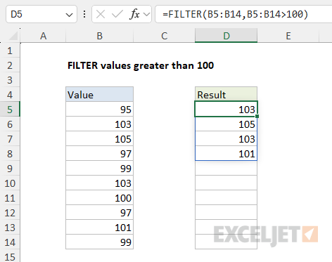
The formula in cell D5 looks like this:

=FILTER(B5:B14,B5:B14>100)

Notice that the include argument is a logical expression, B5:B14. Because there are 10 cells in the range, the expression returns an array that contains 10 results like this:

=FILTER(B5:B14,{FALSE;TRUE;TRUE;FALSE;FALSE;TRUE;FALSE;FALSE;TRUE;FALSE})

Each result in the array corresponds to a value in B5:B14. The FILTER function uses this array to "filter" the values in B5:B14. The values in B5:B14 that are associated with TRUE are returned, and the values associated with FALSE are discarded.

Filter for Red group

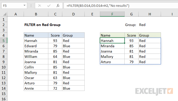
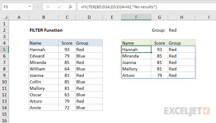
In the example shown above, the formula in F5 is:

=FILTER(B5:D14,D5:D14=H2,"No results")

Since the value in H2 is "Red", the FILTER function extracts data from the array when the Group column equals "Red". All matching records are returned to the worksheet starting from cell F5, where the formula resides.

Values can be hardcoded as well. The formula below has the same result as above with "red" hardcoded into the criteria:

=FILTER(B5:D14,D5:D14="Red","No results")

No matching data

FILTER will return a #CALC! error if no matching data is found, but you can use the optional is_empty argument to return a different result. Often, is_empty is configured to provide a message to the user. For example, the formula below will return "No results" if the logic applied by the include argument fails to match any values:

=FILTER(array,include,"No results") // display message

To display nothing when no matching data is found, provide an empty string ("") for if_empty:

=FILTER(array,include,"") // display nothing

Note that the value for is_empty is only used when FILTER does not find matching results.

Values that contain text

To extract data based on a logical test for values that contain specific text, you can use a formula like this:

=FILTER(rng1,ISNUMBER(SEARCH("txt",rng2)))

In this formula, the SEARCH function is used to look for "txt" in rng2, which would typically be a column in rng1. The ISNUMBER function is used to convert the result from SEARCH into TRUE or FALSE. Read a full explanation here.

Filter by date

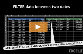
FILTER can be used with dates by constructing logical tests appropriate for Excel dates. For example, to extract records from rng1 where the date in rng2 is in July you can use a generic formula like this:

=FILTER(rng1,MONTH(rng2)=7,"No data") 

This formula relies on the MONTH function to compare the month of dates in rng2 to 7.  See full explanation here.

Multiple criteria

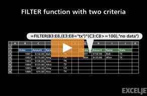
At first glance, it's not obvious how to apply multiple criteria with the FILTER function. Unlike older functions like COUNTIFS and SUMIFS, which provide multiple arguments for entering multiple conditions, the FILTER function only provides a single argument, include, to target data. The trick is to create logical expressions that use Boolean algebra to target the data of interest and supply these expressions as the include argument. For example, to extract data where one value is "A" and another value is greater than 80, you can use a formula like this:

=FILTER(range,(range="A")*(range>80),"No data")

The math operation of multiplication (*) joins the two conditions with AND logic: both conditions must be TRUE in order for FILTER to retrieve the data. See a detailed explanation here.

Complex criteria

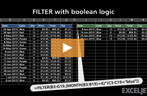
To filter and extract data based on multiple complex criteria, you can use the FILTER function with a chain of expressions that use boolean logic. For example, the generic formula below filters based on three separate conditions: account begins with "x" AND region is "east", and month is NOT April.

=FILTER(data,(LEFT(account)="x")*(region="east")*NOT(MONTH(date)=4))

See this page for a full explanation. Building criteria with logical expressions is an elegant and flexible approach that can be extended to handle many complex scenarios. See below for more examples.

Wildcards

The FILTER function does not support the wildcards (*?~) like the XLOOKUP function. However, you can work around this limitation by combining the FILTER function with the SEARCH function like this:

=FILTER(range,ISNUMBER(SEARCH("substring",range)))

The SEARCH function automatically performs a substring search, and supports wildcards directly if you need more flexibility. See FILTER text contains and Cell contains specific text for a more complete explanation.

Notes

1. FILTER can work with both vertical and horizontal arrays.
2. The include argument must have dimensions compatible with the array argument, or FILTER will return #VALUE!
3. If the include array includes any errors, FILTER will return an error.