SORT Function

The SORT function sorts the contents of a range or array in ascending or descending order. The result is a dynamic array of values that will "spill" onto the worksheet. If values in the source data change, the result from SORT updates automatically. Note that the SORT function cannot sort data in place like Excel's Sort command on the Ribbon. SORT always outputs results to a new location.

By default, SORT sorts values in ascending order using the first column in array. Use sort_index to specify which column (or row) to sort by, and sort_order to control direction: 1 for ascending, -1 for descending. To sort horizontally by columns instead of rows, set by_col to TRUE.

SORT only accepts a single value for sort_index, but you can sort by multiple columns at once using array constants. For example, {1,2} sorts by column 1, then column 2. See the multi-level sort example below. SORT can only sort alphabetically in A-Z or Z-A order. To sort in a custom order (e.g., "High, Medium, Low"), use the SORTBY function instead.

Note that SORT won't automatically adjust the source range if data is added or deleted. To configure SORT with a range that automatically adjusts to fit the data, use an Excel Table or a dynamic range created with TRIMRANGE or the dot operator.

Video: Basic SORT function example

Key features

• Returns a dynamic array that spills automatically
• Sorts rows (default) or columns (set by_col to TRUE)
• Ascending order by default; use -1 for descending
• Handles text, numbers, and dates
• Supports multi-level sorting with array constants
• Works with Excel Tables and structured references

Table of contents

• Basic usage
• Simple A-Z sort
• Sort by specific column
• Sort data horizontally
• Filter on top n values
• Unique rows
• Multi-level sort
• Reverse sort with checkbox
• Dates in chronological order
• Notes

Basic usage

To sort in ascending or descending order:

=SORT(A1:A10) // sort A-Z (ascending)
=SORT(A1:A10,,-1) // Z-A (descending)

To sort by a specific column:

=SORT(A1:B10) // sort by column 1, ascending
=SORT(A1:B10,2) // sort by column 2, ascending
=SORT(A1:B10,2,-1) // sort by column 2, descending

Simple A-Z sort

In its simplest form, the SORT function sorts a single column of data in ascending order. In the worksheet below, the goal is to sort names in column B alphabetically. The formula in D5 is:

=SORT(B5:B16)

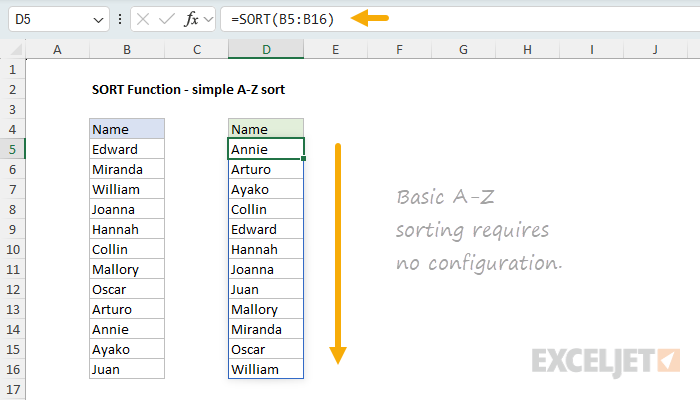
With no optional arguments, SORT returns all values in ascending (A-Z) order. The result spills into D5:D16.

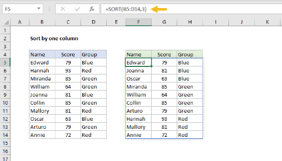
Sort by specific column

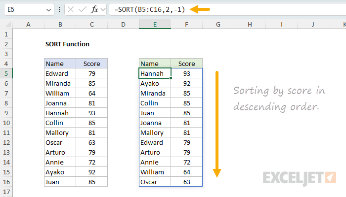
When data has multiple columns, use sort_index to specify which column to sort by. In the worksheet below, the goal is to sort names and scores by score in descending order (highest first). The formula in E5 is:

=SORT(B5:C16,2,-1)

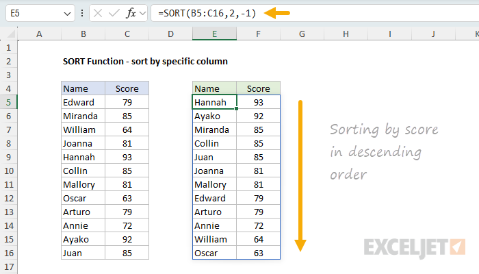
The sort_index of 2 tells SORT to use the second column (Score) for sorting. The sort_order of -1 sorts in descending order. The entire range is returned, sorted by score from highest to lowest. When sort_order is omitted, it defaults to 1 (ascending order).

For more details, see Sort by one column.

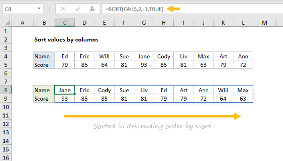
Sort data horizontally

The SORT function has the ability to sort data vertically (by row) or horizontally (by column). To sort data horizontally, set by_col to TRUE. In the worksheet below, names appear in row 4 and scores in row 5. The goal is to sort by score in descending order. The formula in B8 is:

=SORT(B4:K5,2,-1,TRUE)

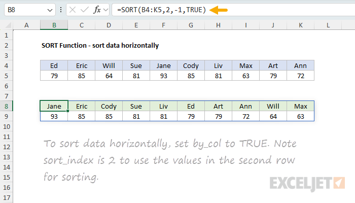
With by_col set to TRUE, the sort_index of 2 refers to row 2 of the array (the scores in row 5). The result is returned horizontally, with names and scores rearranged from highest to lowest score.

For more details, see Sort values by columns.

Filter on top n values

The SORT function pairs well with FILTER to filter and sort data in one step. In the worksheet below, the goal is to extract the top n scores (where n is a variable in cell F2), sorted from highest to lowest. The formula in E5 is:

=SORT(FILTER(B5:C16,C5:C16>=LARGE(C5:C16,F2)),2,-1)

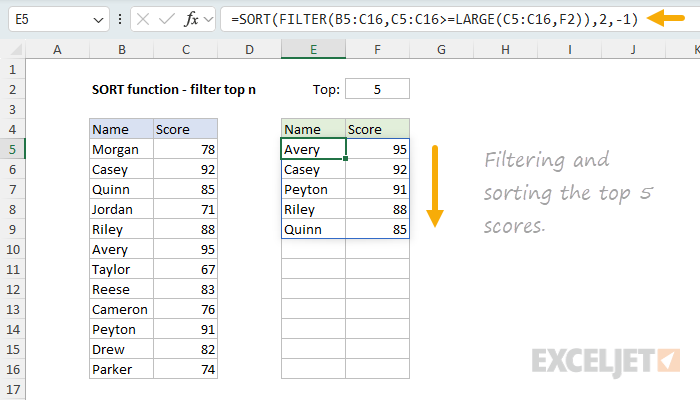
The LARGE function returns the nth largest score (where n comes from F2). FILTER returns all rows where the score is greater than or equal to this value. SORT then sorts the results by column 2 (Score) in descending order. Changing the value in F2 instantly updates the results.

For more details, see Filter on top n values.

Unique rows

The SORT function works well with UNIQUE to extract and sort unique rows. In the worksheet below, the goal is to extract unique Group/Color combinations, sorted by Group. The formula in E5 is:

=SORT(UNIQUE(B5:C16))

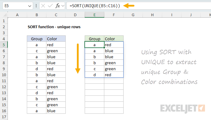
The UNIQUE function extracts unique rows from B5:C16. SORT then sorts these rows by the first column (Group) in ascending order. The result spills into the output range automatically.

For more details, see Unique rows.

Multi-level sort

The SORT function can sort by multiple columns using array constants for sort_index and sort_order. In the worksheet below, the goal is to sort first by Group (ascending), then by Score (descending). The formula in F5 is:

=SORT(B5:D16,{2,3},{1,-1})

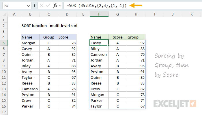
The array constant {2,3} tells SORT to sort first by column 2 (Group), then by column 3 (Score). The array constant {1,-1} specifies ascending order for Group and descending order for Score. Items in Group "A" appear first, sorted by Score from highest to lowest.

For more flexible multi-level sorting, consider the SORTBY function, which lets you sort by columns that aren't part of the source data.

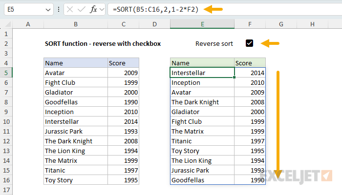
Reverse sort with checkbox

You can use a checkbox (or any TRUE/FALSE value) to toggle between ascending and descending sort order. In this example, movie titles are sorted from oldest to newest by default using the release year in the second column. Cell F2 contains a checkbox labeled "Reverse sort". The formula in E5 is:

=SORT(B5:C16,2,1-2*F2)

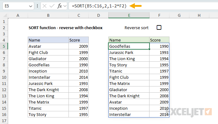
In Excel, a checkbox returns a TRUE/FALSE value. When the checkbox is unchecked, the value is FALSE. When the checkbox is checked, the value is TRUE. The expression 1-2*F2 is a simple trick to convert TRUE/FALSE to the sort order values SORT expects:

• When F2 is FALSE (unchecked): 1-2*0 = 1 (ascending)
• When F2 is TRUE (checked): 1-2*1 = -1 (descending)

Clicking the checkbox instantly reverses the sort order:

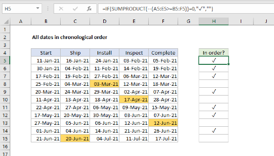
Dates in chronological order

The SORT function can be used to validate whether data is sorted correctly. For example, in the worksheet below, each row contains project milestone dates: Start, Ship, Install, Inspect, and Complete. The goal is to verify that all dates in a row are in the correct sequence. The formula in H5 is:

=IF(SUM(--(B5:F5<>SORT(B5:F5,1,1,1)))=0,"✓","")

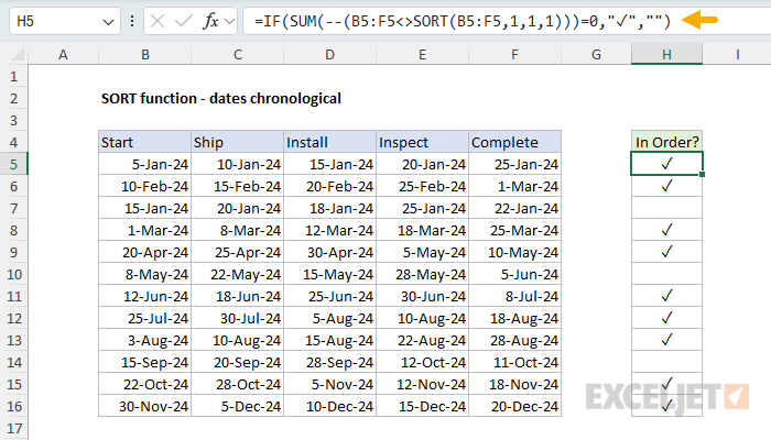
The formula compares each date in B5:F5 to the same dates after sorting horizontally with SORT (the final argument of 1 sets by_col to TRUE for horizontal sorting). The double-negative (--) converts the TRUE/FALSE values to 1/0, and the SUM function counts how many dates are different after sorting. If the count is zero, all dates are listed chronologically and a check mark (✓) is returned.

For more details, see All dates in chronological order.

Notes

• SORT returns a #VALUE! error if sort_index is out of range.
• SORT returns a #SPILL! error if the spill range is not empty.
• SORT returns a #REF! error when referencing a closed workbook (dynamic arrays require open workbooks).
• SORT is a "stable sort"—items with the same sort value maintain their original relative order.
• Do not include headers in the array argument; SORT treats all rows as data.
• SORT works with Excel Tables and structured references. Results update automatically when table data changes.
• Use the SORTBY function to sort data by values that are not part of the data being sorted.