Summary
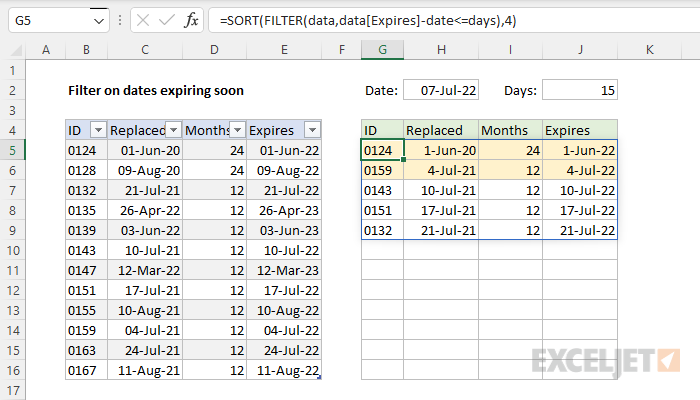
To filter a set of data to show rows where dates are expiring soon (or have already expired) you can use the FILTER function with the SORT function. In the example shown, the formula in G5 is:
=SORT(FILTER(data,data[Expires]-date<=days),4)
where data is an Excel Table in the range B5:E16, and date (H2) and days (J2) are named ranges. The result is the five rows in the table with an expiration date within the next 15 days:
Explanation
In this example, the goal is to filter data to show rows where dates have expired or will be expiring soon. In the table to the left, we have equipment that needs to be replaced every x months, where x appears in the "Months" column. The "Replaced" column shows the date equipment was replaced. The "Expires" column shows the date it will need to be replaced again.
All data is in an Excel Table named data in the range B5:E16 and the dates to check are in the "Expires" column. In addition, the current date is in the named range date (H2) and the number of days to use when deciding if a date is expiring soon is in the named range days (J2). Dates already expired are highlighted in yellow with conditional formatting. The named ranges are for convenience only, to make the formula easier to read and write.
You can use this same approach to filter on any data that has an upcoming date. i.e. retirements, events, renewals, etc.
Note: In the example shown, the current date is 7-July-2022, provided by the TODAY function. As time goes by, the current date will move forward, and more dates will be expired or expiring soon. To see the worksheet in its original state, you can hardcode the date 7-July-2022 into cell H2.
The core logic
In the example shown, the formula in G5 is:
=SORT(FILTER(data,data[Expires]-date<=days),4)
Working from the inside out, the core logic in this formula first works out the difference between the value in date (H2) and all dates in column E:
data[Expires]-date<=days)
Because Excel dates are just large serial numbers, we simply subtract the value in date from each date in the Expires column. When the expiration date is in the past, the result is a negative number. When the expiration date is in the future, the result date is a positive number. In the example shown:
data[Expires]-date
returns the following array:
{-36;33;14;293;331;3;248;10;34;-3;17;35}
Each number represents the number of days until expiration. Again, negative numbers are dates already expired. When this array is compared to days (J2) which is 15:
={-36;33;14;293;331;3;248;10;34;-3;17;35}<=15
the result is an array of TRUE and FALSE values like this:
{TRUE;FALSE;TRUE;FALSE;FALSE;TRUE;FALSE;TRUE;FALSE;TRUE;FALSE;FALSE}
Each TRUE value represents a date that has already expired or will expire in the next 15 days. We can use this same logic in the FILTER function to select dates expiring soon.
FILTER function
The next step is to implement the logic above inside the FILTER function. To filter the dates to show those expiring within 15 days, we embed the expression explained above inside FILTER like this:
FILTER(data,data[Expires]-date<=days)
The array argument is the Excel Table data, and the include argument is the logical expression explained above. In this configuration, FILTER returns the five rows from the table where the Expires date has already occurred or will occur in the next 15 days. Note that this result is based on the current date in cell H2, which is 7-July-2022.
SORT function
The final step in the problem is to sort the data by expiration date, so that dates already expired are listed first, followed by dates expiring soon in the order they will expire. This can be done by nesting the FILTER formula inside the SORT function like this:
=SORT(FILTER(data,data[Expires]-date<=days),4)
Here, the array provided to SORT is the result returned by FILTER, and sort_index is given as 4, since the "Expires" date is in the fourth column of the table.
Current date
In the worksheet shown, the current date is provided by the TODAY function:
=TODAY()
TODAY takes no arguments, and will return the current date on an ongoing basis. This is often what you want in real life, where the data being tracked is always changing. However, it can be confusing in the case of this example, because the worksheet in the future will not look the same as the worksheet looks today. To make the worksheet look like it did on July 7, 2022, just hardcode that date into cell H2.
Conditional formatting
In the example shown, conditional formatting is used to highlight dates that have already expired. The formula used to apply the rule is based on the AND function:
=AND($J5<>"",$J5<=date)
In this formula, we check two conditions: (1) the date in J5 is not empty and (2) the date in J5 is less than or equal to (<=) date (H2), which holds the current date. This is an example of a mixed reference – the column is locked in order to highlight the entire row.
Expires date
The date in the "Expires" column is calculated with the EDATE function. The formula in E5 is:
=EDATE(C5,D5)
Starting with the "Replaced" date, EDATE returns moves forward the number of months given in "Months" and returns the resulting date.