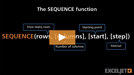
=SEQUENCE(rows, [columns], [start], [step])- rows - Number of rows to return.
- columns - [optional] Number of columns to return.
- start - [optional] Starting value (defaults to 1).
- step - [optional] Increment between each value (defaults to 1).
Using the SEQUENCE function
The SEQUENCE function generates a list of sequential numbers in an array. The array can be one-dimensional or two-dimensional, controlled by the rows and columns arguments. On its own, SEQUENCE creates numbers that spill onto the worksheet: row numbers, a list of dates, or a calendar. Inside another formula, SEQUENCE supplies a list of numbers that the formula needs, a requirement that comes up constantly in more advanced formulas.
SEQUENCE is a key piece of Excel's support for dynamic arrays, so you will see it appear in an astonishing number of other formulas. For this reason, it is important to understand how the SEQUENCE function works.
SEQUENCE takes four arguments: rows, columns, start, and step. The rows and columns arguments set the size of the output, start is the first number, and step is the increment between numbers. The columns, start, and step arguments are optional and default to 1.
Video: The SEQUENCE function
Key features
- Returns a list of numbers in a column, a row, or a two-dimensional grid.
- The columns, start, and step arguments default to 1.
- step can be negative to count down, zero to repeat one value, or a decimal.
- A grid fills across each row first, then moves down to the next row.
- rows and columns can come from other formulas (ROWS, COUNTA, LEN), so the output resizes with your data.
- Dates and times in Excel are numbers, so SEQUENCE creates date and time lists directly.
- Often used inside other formulas, where it supplies a list of positions or counts.
Table of contents
- Basic examples
- Number rows automatically
- Fill a grid down columns
- List all dates in a month
- Monthly and quarterly dates
- List workdays
- Dynamic calendar
- Letters A to Z
- Sum top n values
- Split text into characters
- Reverse a text string
- Reverse a list
- Random numbers without duplicates
- Every nth row
- Repeat a range of values
- SEQUENCE versus ROW and INDIRECT
- Notes
Basic examples
The output from SEQUENCE is an array of numbers. For example, the formulas below each create an array of numbers between 1 and 5:
=SEQUENCE(5,1) // returns {1;2;3;4;5} in 5 rows
=SEQUENCE(1,5) // returns {1,2,3,4,5} in 5 columns
The formula below will create a 5 x 5 array that contains 25 cells with the values 1-25:
=SEQUENCE(5,5) // numbers 1-25 in a 5 x 5 array
Either rows or columns can be omitted:
=SEQUENCE(5) // returns {1;2;3;4;5} in 5 rows
=SEQUENCE(,5) // returns {1,2,3,4,5} in 5 columns
The start argument is the starting point in the numeric sequence, and step controls the increment between each value. Both formulas below use a start value of 10 and a step value of 5:
=SEQUENCE(3,1,10,5) // returns {10;15;20} in 3 rows
=SEQUENCE(1,3,10,5) // returns {10,15,20} in 3 columns
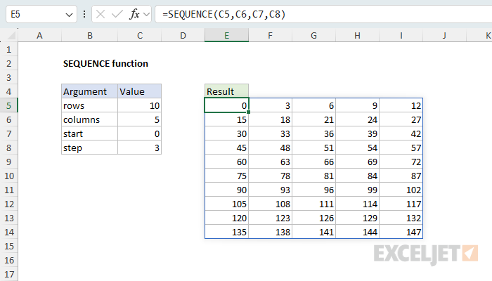
In the worksheet shown above, SEQUENCE takes all four arguments from cells, and the formula in E5 is =SEQUENCE(C5,C6,C7,C8). The result is 10 rows and 5 columns of numbers that start at 0 and increase by 3, ending at 147. The formulas below show a few more configurations:
=SEQUENCE(100) // 1 to 100
=SEQUENCE(100,,100,-1) // 100 to 1 with negative step
=SEQUENCE(5,,1,0) // {1;1;1;1;1}, start at 1, step 0
=SEQUENCE(7,1,DATE(2026,1,1)) // 7 days from January 1, 2026
=SEQUENCE(12,1,TIME(8,0,0),TIME(1,0,0)) // hourly times from 8:00 AM
The date and time results display as plain numbers until you apply a date or time number format.
Number rows automatically
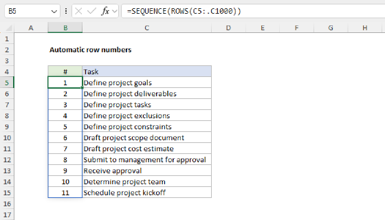
A common need is to number the rows in a list, and to have the numbers extend automatically when the list grows. In the worksheet below, names are in column C, and the formula in B5 is:
=SEQUENCE(ROWS(C5:.C1000))
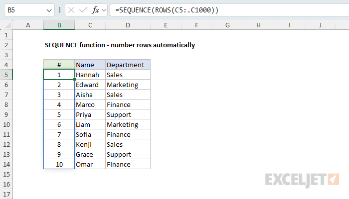
The range C5:.C1000 is a trim reference: the dot after the colon tells Excel to trim empty rows from the end of the range. With 10 names in column C, the trimmed range is C5:C14, the ROWS function returns 10, and SEQUENCE returns the numbers 1 to 10, which spill into B5:B14. Add a name in C15, and the trimmed range grows to C5:C15, so a new row number appears. Remove a name, and the numbers shrink to match. You can also trim the range with the TRIMRANGE function, which gives the same result here:
=SEQUENCE(ROWS(TRIMRANGE(C5:C1000)))
Trim references and TRIMRANGE are available in Excel 365 only. In other versions, you can count the names with the COUNTA function instead:
=SEQUENCE(COUNTA(C5:C1000))
The difference shows up when the list has a blank cell. COUNTA counts only cells that aren't empty, so one blank in the list leaves the last name without a number. A trim reference only trims empty rows at the end of the range, so a blank row inside the list still gets a number, and the numbers stay lined up with the names. One catch: if the list is completely empty, the trim reference returns a #REF! error.
SEQUENCE can't spill inside an Excel Table. For row numbers in a table, and other options, see Automatic row numbers.
Fill a grid down columns
When SEQUENCE creates a two-dimensional array, it fills across each row first, then moves down to the next row. What if you want the numbers to run down each column instead? In the worksheet below, the formula in B5 fills across, and the formula in G5 fills down:
=SEQUENCE(5,4) // fill across
=WRAPCOLS(SEQUENCE(20),5) // fill down
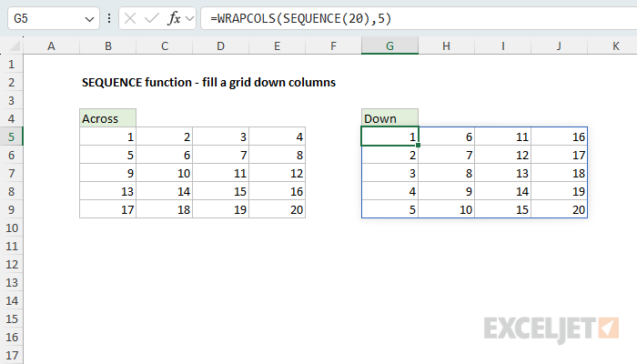
SEQUENCE(20) returns the numbers 1 to 20 in a single column, and the WRAPCOLS function wraps that column into columns of 5 values each. The result is the same 5 x 4 grid, filled down instead of across. WRAPCOLS is available in Excel 2024+ and Excel 365. In Excel 2021, you can get the same result with the TRANSPOSE function: create the grid with rows and columns swapped, then flip it:
=TRANSPOSE(SEQUENCE(4,5))
List all dates in a month
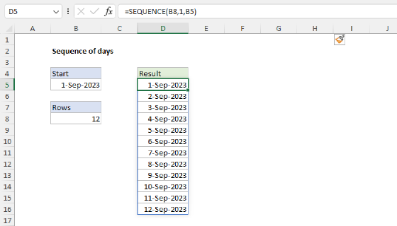
Because Excel dates are serial numbers, SEQUENCE can generate a list of dates directly. For example, to list 12 consecutive days starting with a date in B5:
=SEQUENCE(12,1,B5)
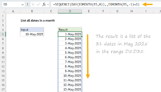
To list all the dates in a month, you need two more pieces of information: the number of days in the month, and the first day of the month. In the worksheet below, B5 contains February 15, 2026, and the formula in D5 is:
=SEQUENCE(DAY(EOMONTH(B5,0)),,EOMONTH(B5,-1)+1)
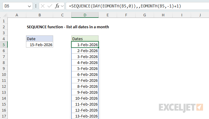
The EOMONTH function does most of the work. EOMONTH(B5,0) returns the last day of the month, February 28, 2026, and the DAY function returns its day number, 28, which becomes rows. EOMONTH(B5,-1)+1 returns the last day of the previous month plus one day, February 1, 2026, which becomes start. SEQUENCE returns 28 dates beginning February 1, which spill into D5:D32. Enter a date in a different month in B5, and the list updates.
SEQUENCE returns raw numbers only. Apply date formatting to display a date.
For more details, see List all dates in a month. To list a given number of days from a start date, see Sequence of days.
Monthly and quarterly dates
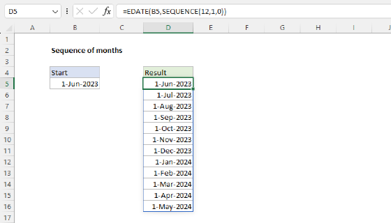
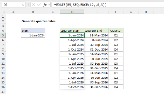
Months have different lengths, so you can't step through months by adding a fixed number of days. Instead, use SEQUENCE to create month offsets, and let the EDATE function do the date math. In the worksheet below, the start date is in B5, and the formulas in D5 and F5 are:
=EDATE(B5,SEQUENCE(12,1,0)) // monthly
=EDATE(B5,SEQUENCE(4,1,0,3)) // quarterly
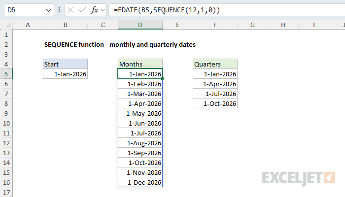
In both formulas, SEQUENCE generates an array of numbers that EDATE uses for the months argument, so each number is an offset from the start date. In the first formula, SEQUENCE returns the offsets 0 to 11:
{0;1;2;3;4;5;6;7;8;9;10;11}
EDATE adds each offset to the start date as a number of months, so the result is 12 dates, one month apart, beginning January 1, 2026. A start of 0 means the list begins with the start date itself. In the second formula, a step of 3 returns {0;3;6;9}, so EDATE returns four dates, one quarter apart. To display month names instead of dates, apply a custom number format like "mmmm", or wrap the formula in the TEXT function:
=TEXT(EDATE(B5,SEQUENCE(12,1,0)),"mmmm")
For more details, see Sequence of months and Generate quarter dates. To step by years, see Sequence of years.
List workdays
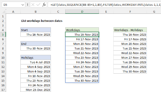
To list workdays and skip weekends and holidays, you can use SEQUENCE with the WORKDAY.INTL function. In the worksheet below, the start date is in B5, the holidays are in F5:F6, and the formula in D5 is:
=WORKDAY.INTL(B5-1,SEQUENCE(12),1,F5:F6)
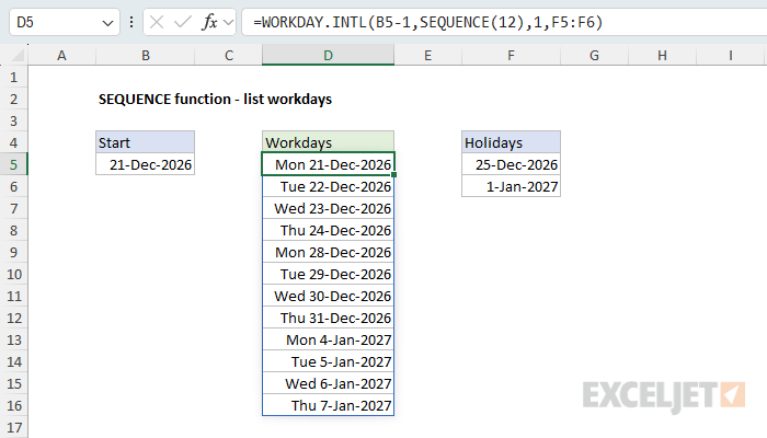
WORKDAY.INTL returns the date that is a given number of workdays after a start date. SEQUENCE(12) supplies the numbers 1 to 12, so WORKDAY.INTL returns 12 working days based on the start date. Subtracting 1 from B5 moves the starting point back one day, so the list begins with the start date itself when it is a workday. The weekend argument, 1, makes Saturday and Sunday the weekend, and the dates in F5:F6 are skipped as holidays. The result is 12 workdays from Monday, December 21, 2026, through Thursday, January 7, 2027, without Christmas Day or New Year's Day.
To handle a custom work schedule, change the weekend code. For example, 11 makes Sunday the only weekend day, and a text code like "0000111" makes Friday, Saturday, and Sunday weekend days (one digit per day, starting with Monday). For more details, see Sequence of workdays. For weekends only or a custom set of days, see Sequence of weekends and Sequence of custom days.
Dynamic calendar
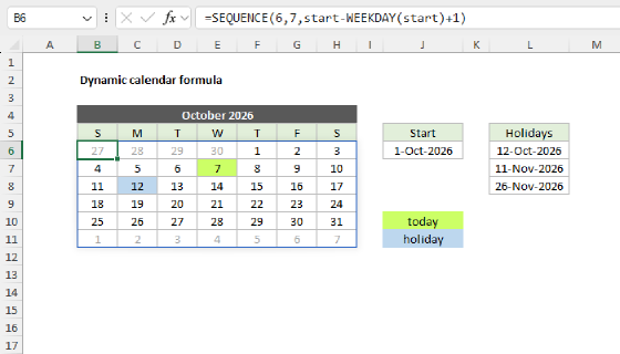
A monthly calendar is a grid of dates 7 columns wide and 6 rows tall, which makes it a natural fit for SEQUENCE. In the worksheet below, B5 contains the first day of the month, and the formula in D5 is:
=SEQUENCE(6,7,B5-WEEKDAY(B5)+1)
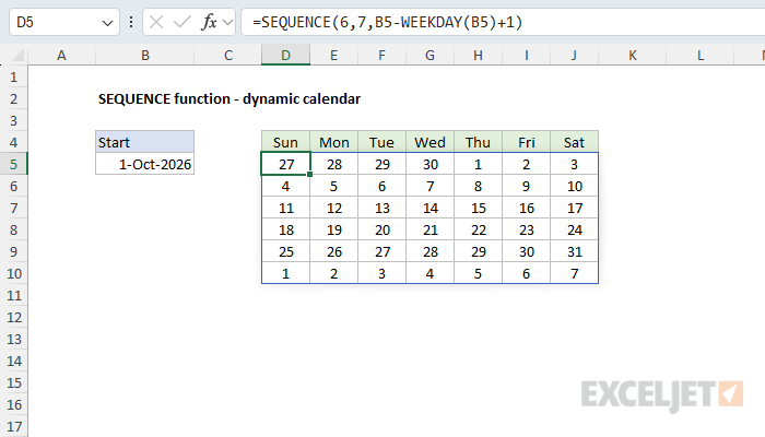
The trick is the start value. A calendar whose weeks start on Sunday needs to begin with the Sunday on or before the first of the month. The WEEKDAY function returns 1 for Sunday through 7 for Saturday, so B5-WEEKDAY(B5)+1 steps back to the previous Sunday. October 1, 2026, is a Thursday (weekday 5), so the calendar starts on September 27, 2026. SEQUENCE returns 42 consecutive dates in 6 rows of 7, and the number format "d" displays the day number only. Enter a different first-of-month date in B5, and the calendar redraws.
Notice that the grid includes days from September and November. The full example uses conditional formatting to dim those days and to highlight holidays. For details, see Dynamic calendar formula.
Letters A to Z
SEQUENCE only returns numbers, but other functions can turn numbers into text. In the worksheet below, the formulas in B5 and D5 return the letters of the alphabet:
=CHAR(SEQUENCE(26,,65)) // A to Z
=CHAR(SEQUENCE(26,,97)) // a to z
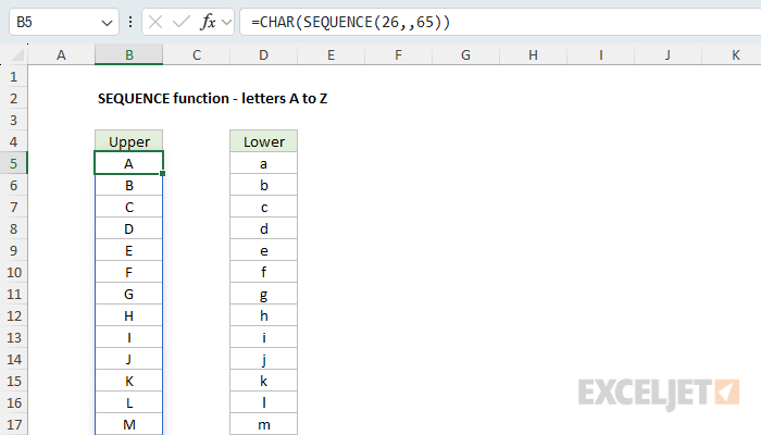
This works because every character has a numeric code, and the CHAR function converts a code back into its character. SEQUENCE(26,,65) returns 26 numbers starting at 65, and CHAR converts each number into the character with that ASCII code. The letter "A" is 65, "Z" is 90, and the lowercase letters start at 97. To list the letters across a row instead, set rows to 1 and columns to 26:
=CHAR(SEQUENCE(1,26,65)) // A to Z in a row
For an example that uses this idea to build random text, see Generate random text strings.
Sum top n values
In this example, the output from SEQUENCE never appears on the worksheet. Instead, SEQUENCE creates a list of numbers that another function needs. The goal is to sum the top n scores, where n is entered in D5. The formula in E5 is:
=SUM(LARGE(B5:B16,SEQUENCE(D5)))
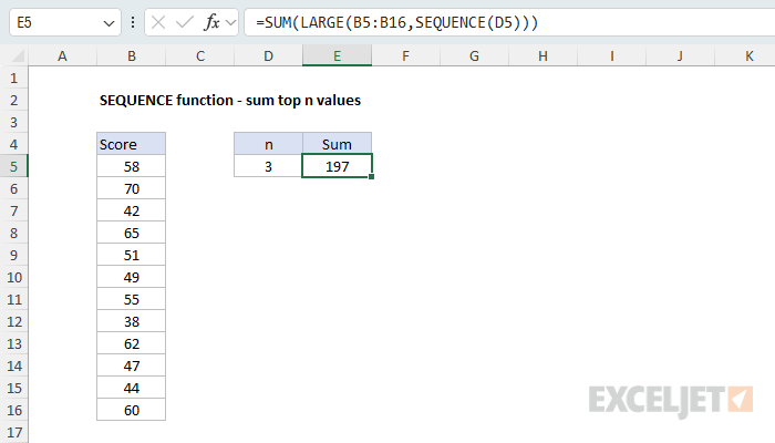
The LARGE function returns the nth largest value in a range, where n is given by the k argument. When k is an array, LARGE returns one result for each value in the array. With 3 in D5, SEQUENCE returns {1;2;3}:
=SUM(LARGE(B5:B16,{1;2;3}))
LARGE returns the 1st, 2nd, and 3rd largest scores, {70;65;62}, and the SUM function adds them up to get 197. Change n in D5, and SEQUENCE returns a different number of values. To sum the bottom n values, use the SMALL function instead. For more details, see Sum top n values, Sum bottom n values, and Average top 3 scores.
Split text into characters
To split a text string into individual characters, you can combine SEQUENCE with the MID function. In the worksheet below, the formula in D5, copied down, is:
=MID(B5,SEQUENCE(1,LEN(B5)),1)
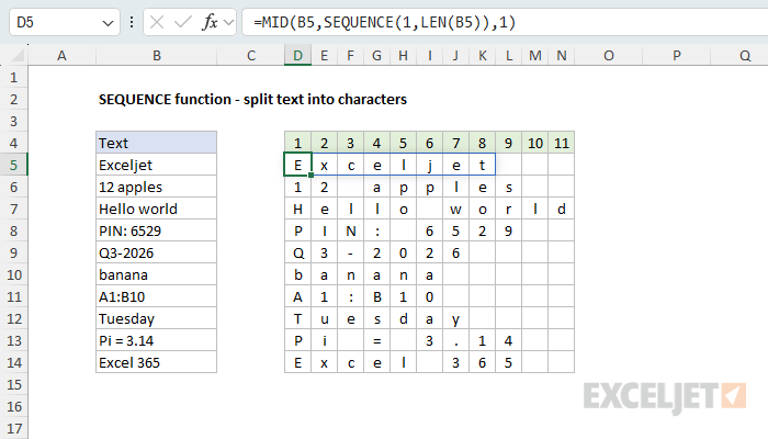
The LEN function returns the number of characters in B5, and SEQUENCE uses that count to create a horizontal array of positions. "Exceljet" has 8 characters, so SEQUENCE returns {1,2,3,4,5,6,7,8}:
=MID(B5,{1,2,3,4,5,6,7,8},1)
MID extracts 1 character at each position and returns {"E","x","c","e","l","j","e","t"}, which spills across the row. Setting rows to 1 and columns to the length makes the result horizontal; SEQUENCE(LEN(B5)) returns a vertical list instead. This MID and SEQUENCE pattern is the basis of many text formulas, including the next example.
In Excel 365, the REGEXEXTRACT function can split text into characters directly with
=REGEXEXTRACT(B5,".",1). For details on both approaches, see Split text string to character array.
Reverse a text string
Building on the previous example, you can reverse a text string by extracting the characters in reverse order and joining them back together. In the worksheet below, the formula in D5, copied down, is:
=CONCAT(MID(B5,SEQUENCE(LEN(B5),,LEN(B5),-1),1))
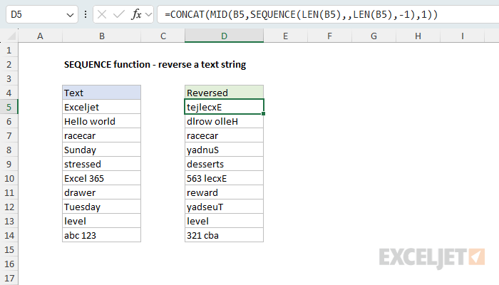
This time, SEQUENCE uses LEN(B5) twice: once for rows, and once for start. With a step of -1, SEQUENCE counts down from the last character to the first. For "Exceljet", the result is {8;7;6;5;4;3;2;1}:
=CONCAT(MID(B5,{8;7;6;5;4;3;2;1},1))
MID returns the characters in reverse order, and the CONCAT function joins them into a single text string, "tejlecxE". If B5 is empty, LEN returns zero and the formula returns #CALC!. For more details, see Reverse text string.
Reverse a list
To reverse the order of a list, you can use SEQUENCE to create a sort key for the SORTBY function. In the worksheet below, the formula in D5 is:
=SORTBY(B5:B14,SEQUENCE(ROWS(B5:B14)),-1)
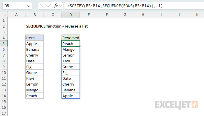
The ROWS function returns 10, and SEQUENCE returns the numbers 1 to 10, one for each item in the list:
=SORTBY(B5:B14,{1;2;3;4;5;6;7;8;9;10},-1)
These numbers are the original position of each item in the list. SORTBY sorts the list by position in descending order (-1), so the last item comes first and the first item comes last. For more details, see Reverse a list or range.
Random numbers without duplicates
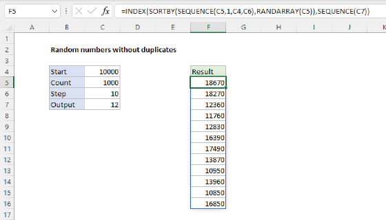
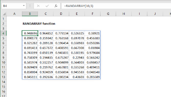
The RANDARRAY function can generate random whole numbers, but nothing stops it from returning duplicates. To draw random numbers with no duplicates, like a raffle, you can shuffle a list created by SEQUENCE. In the worksheet below, the formula in B5 is:
=TAKE(SORTBY(SEQUENCE(50),RANDARRAY(50)),10)
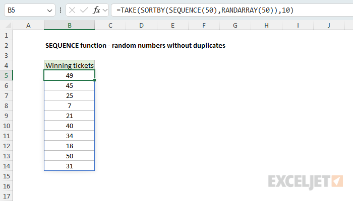
SEQUENCE(50) returns the numbers 1 to 50, and RANDARRAY(50) returns 50 random decimal values. SORTBY sorts the numbers by the random values, which shuffles them into a random order. Every number from 1 to 50 appears exactly once, so the shuffled list can't contain duplicates. Finally, the TAKE function returns the first 10 numbers, which are the winning tickets. TAKE is available in Excel 2024+ and Excel 365.
RANDARRAY is a volatile function, so the draw changes every time the worksheet recalculates. For random results that only change when you change a seed value, see Seeded random number generator in Excel (Excel 365). For more details, and a version with a custom start and step, see Random numbers without duplicates. To shuffle people into random groups, see Randomly assign people to groups.
Every nth row
To extract every nth row from a range, you can use SEQUENCE with the MOD function and the FILTER function. In the worksheet below, the formula in E5 returns every third row from the data in B5:C16:
=FILTER(B5:C16,MOD(SEQUENCE(ROWS(B5:B16)),3)=0)
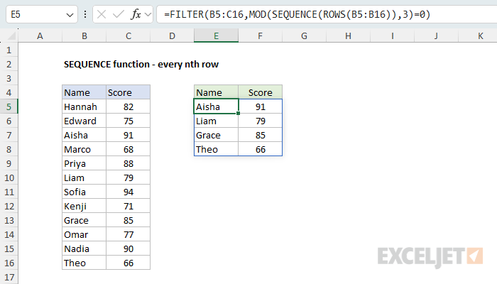
SEQUENCE(ROWS(B5:B16)) returns the numbers 1 to 12, one for each row in the data. These are positions inside the range, not worksheet row numbers, so the formula works wherever the data sits. MOD returns the remainder after dividing each number by 3, which is zero for every third row:
MOD({1;2;3;4;5;6;7;8;9;10;11;12},3) // returns {1;2;0;1;2;0;1;2;0;1;2;0}
Comparing the remainders to zero creates an array of TRUE and FALSE values, and FILTER returns the rows where the value is TRUE: rows 3, 6, 9, and 12. To return every 2nd or 4th row, change 3 to 2 or 4. For more details, see Filter every nth row. The same idea works for math on every nth value: see Sum every nth row, Sum every nth column, and Max of every nth column.
Repeat a range of values
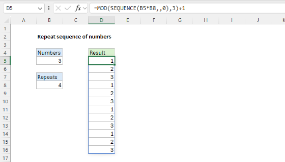
To repeat a list of values, you can use SEQUENCE and MOD to create a repeating pattern of index numbers. In the worksheet below, the formula in D5 repeats the three colors in B5:B7 four times:
=CHOOSEROWS(B5:B7,MOD(SEQUENCE(12,,0),3)+1)
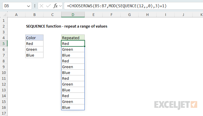
SEQUENCE(12,,0) returns 12 numbers starting at zero. MOD divides each number by 3 and returns the remainder, which cycles through 0, 1, and 2. Adding 1 shifts the cycle to 1, 2, and 3:
MOD(SEQUENCE(12,,0),3)+1 // returns {1;2;3;1;2;3;1;2;3;1;2;3}
The CHOOSEROWS function returns the rows of B5:B7 in this order, so the three colors repeat four times. Starting SEQUENCE at zero is what makes the pattern begin with 1. To repeat the values a different number of times, change 12 to another multiple of 3. CHOOSEROWS is available in Excel 2024+ and Excel 365. For more details, see Repeat range of values. To repeat numbers instead of values, see Repeat sequence of numbers.
SEQUENCE versus ROW and INDIRECT
Before SEQUENCE, Excel had no function to directly generate a list of numbers, so formulas used workarounds based on the ROW function. You will still see these patterns in forum answers and older formulas, including some pages on this site:
=ROW(INDIRECT("1:"&n)) // numbers 1 to n
=ROW(A1:A10)-ROW(A1)+1 // numbers 1 to 10
Both formulas work, but they are harder to read, and each has a weakness:
- The INDIRECT function is volatile, so any formula that uses it recalculates whenever anything in the workbook changes.
ROW(A1:A10)depends on a real range, so inserting or deleting rows inside that range changes how many numbers it returns.
Here are the SEQUENCE equivalents:
=SEQUENCE(n) // numbers 1 to n
=SEQUENCE(10) // numbers 1 to 10
SEQUENCE isn't volatile and doesn't depend on a cell reference, so if you have SEQUENCE, you don't need either pattern.
Notes
- If the cells where the result should spill aren't empty, SEQUENCE returns #SPILL!. SEQUENCE also returns #SPILL! inside an Excel Table, because tables don't support spilling formulas.
- If rows or columns is zero, SEQUENCE returns #CALC!. Negative values return #VALUE!, and decimal values are truncated, so
SEQUENCE(2.7)returns{1;2}. - A decimal step can introduce tiny floating-point errors. For example, the 12th value from
=SEQUENCE(12,1,TIME(8,0,0),TIME(1,0,0))displays as 7:00 PM but isn't exactly equal toTIME(19,0,0). When an exact match matters, generate whole numbers and convert them:=TIME(SEQUENCE(12,1,8),0,0)returns exact hours, and=ROUND(SEQUENCE(11,1,0,0.1),1)returns exact tenths. For times that don't start on the hour, round to the nearest minute, as shown in Sequence of times. - A step of zero returns an array of identical values.
SEQUENCE(5,1,1,0)returns{1;1;1;1;1}, a trick used with MMULT to get row totals. - SEQUENCE doesn't return one sequence per value when an argument is an array.
SEQUENCE({3;2})returns{1;1}, the first value of each sequence, not two sequences. To build an array from a custom calculation, see the MAKEARRAY function. - The result must fit on the worksheet.
SEQUENCE(1,17000)returns #SPILL!, because a worksheet has 16,384 columns, and a rows value over 1,048,576 returns #VALUE!. - SEQUENCE returns plain numbers, so dates and times need a date or time number format to display correctly.
- SEQUENCE is available in Excel 2021+ and Excel 365.