Summary
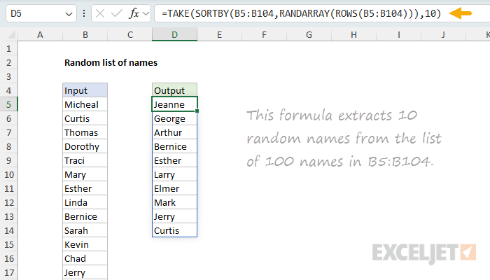
To create a random list of names, you can use a formula based on the TAKE function, SORTBY function, and the RANDARRAY function. In the example shown, the formula in D5 is:
=TAKE(SORTBY(B5:B104,RANDARRAY(ROWS(B5:B104))),10)
The result is a random list of 10 names from the list of 100 names in column B.
Generic formula
=TAKE(SORTBY(names,RANDARRAY(ROWS(names))),n)
Explanation
In this example, the goal is to create a list of 10 random names from a larger list of 100 names. In other words, we want to select a random subset of names from a larger list. The names to select from are in column B, starting in row 5. The formula should handle any number of names in the input list and handle the number of names to select as a variable.
This is an interesting problem in Excel. Although there are several functions dedicated to generating random numbers, including RAND, RANDARRAY, and RANDBETWEEN, it isn't obvious how you would use the output from these functions to generate a random list of names.
This article looks at two formula options to solve this problem. The first option involves sorting all 100 names in a random order, then selecting the first 10 names from the sorted list. The second option generates a list of 10 random integers between 1 and 100, then uses these numbers as indices to select the names in the original list. To start off, let's look at how we can simply sort the names in a random order.
Table of contents
- Sorting names in a random order
- Option 1: TAKE with SORTBY and RANDARRAY
- Option 2: INDEX with RANDARRAY
- Sampling with and without replacement
- Summary and recommendation
Sorting names in a random order
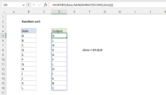
To sort the names in a random order, we can use the SORTBY function and the RANDARRAY function. You can see how this works in the worksheet below, where the formula in D5 is:
=SORTBY(B5:B104,RANDARRAY(ROWS(B5:B104)))
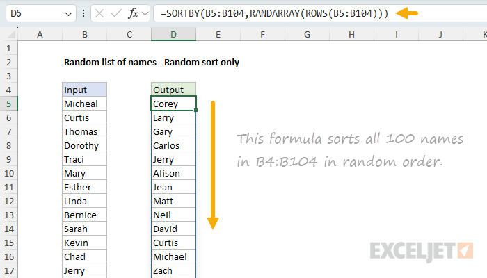
This formula sorts all 100 names in B4:B104 in random order.
Working from the inside out, the ROWS function is used to get the number of rows in the range B5:B104 (100), which is returned to the RANDARRAY function as the rows argument. This determines the number of random numbers to create:
=RANDARRAY(ROWS(B5:B104))
=RANDARRAY(100) // generates 100 random numbers
Next, the RANDARRAY function creates an array of 100 random numbers between 0 and 1. These are long decimals that look something like this:
{0.909292521,0.69722143,0.839223233,0.837319958,0.097171021,...}
In the screenshot below, you can see a full set of 100 random numbers in column D. These are the numbers that will be used to sort the names in a random order.
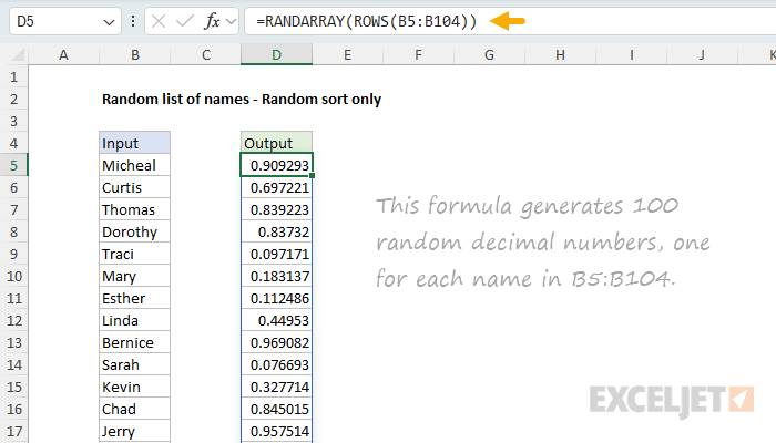
This formula generates 100 random decimal numbers, one for each name in B5:B104.
Next, the array of random numbers created by the RANDARRAY function is returned to the SORTBY function as the sort_by argument:
=SORTBY(B5:B104,{0.909292521,0.69722143,0.839223233,0.837319958,0.097171021,...})
The SORTBY function then sorts the input list by the random array of numbers. The result is a list of names in a random order.
This formula is generally useful to sort any range of values in a random order. Next, let's look at how we can use it to generate 10 random names from the list of 100 names.
Note: the RANDARRAY function is a volatile function and will recalculate every time the worksheet is changed, causing values to be resorted. To stop values from sorting automatically, you can copy the formulas, then use Paste Special > Values to convert formulas to static values. Another option is to adapt the formula to use a this seeded random number generator. This involves replacing RANDARRAY with the custom RAND_SEQUENCE function explained in the article.
Option 1: TAKE with SORTBY and RANDARRAY
Option 1 involves selecting the first 10 names from a randomly sorted list. To sort the list in a random order, we use the SORTBY function with the RANDARRAY function as explained in the previous section. Then, we use the TAKE function to select the first 10 names from the sorted list. You can see this approach in the worksheet below, where the formula in D5 is:
=TAKE(SORTBY(B5:B104,RANDARRAY(ROWS(B5:B104))),10)
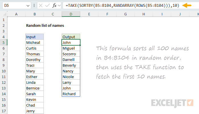
This formula sorts all 100 names in B4:B104 in random order, then uses the TAKE function to fetch the first 10 names in the sorted list.
Working from the inside out, we use SORTBY with RANDARRAY to sort the names in a random order as explained above:
=SORTBY(B5:B104,RANDARRAY(ROWS(B5:B104))) // randomly sort all names
The result from SORTBY is a list of all 100 names in a randomly sorted order.
Finally, we need to retrieve 10 names. Because we already have names in a random order, we can simply ask the TAKE function to fetch the first 10 names in the sorted list:
=TAKE(randomly_sorted_names,10)
Because the input list was sorted randomly, the result from TAKE is a random list of 10 names. I like this approach because it is simple and a great example of how new functions like TAKE can be useful. Let's look at another approach to this problem.
Option 2: INDEX with RANDARRAY
Another way to solve this problem is to generate an array of random integers and then use the INDEX function to select the names at these positions, without sorting the names first. You can see this approach in the worksheet below, where the formula in D5 looks like this:
=INDEX(B5:B104,RANDARRAY(10,1,1,ROWS(B5:B104),1))
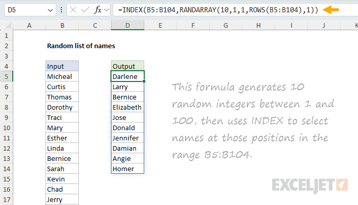
This formula generates 10 random integers between 1 and 100, then uses INDEX to select names at those positions in the range B5:B104.
As before, the ROWS function is used to count the names in the input. However, in this case, the output from ROWS is delivered to RANDARRAY as the max argument, which determines the maximum value for the random numbers to generate.
=RANDARRAY(10,1,1,ROWS(B5:B104),1)
The complete configuration of RANDARRAY is as follows:
- rows: 10
- columns: 1
- min: 1
- max: 100 (from
ROWS(B5:B104)) - integer: TRUE
The result from RANDARRAY is an array of 10 random integers between 1 and 100, like this:
{95;81;6;90;88;82;85;5;82;46}
This array is returned directly to the INDEX function as the row argument:
=INDEX(B5:B104,{95;81;6;90;88;82;85;5;82;46})
Because we give INDEX an array of 10 row numbers, it will return an array of 10 results, each corresponding to a name at the given position:
{"Darlene";"Larry";"Bernice";"Elizabeth";"Jose";"Donald";"Jennifer";"Damian";"Angie";"Homer"}
The final result is a random list of 10 names extracted from the list of 100 names in B5:B104. This approach is more efficient than Option 1 because it does not need to sort the entire list of 100 names. Instead, it creates only as many random integers as we need, then uses those numbers directly to extract names in that position from the master list. However, it comes with a caveat: there is no guarantee that the random integers created by RANDARRAY will be unique, and duplicate integers will result in duplicate names.
Note we are using INDEX and not TAKE to extract names in option 2. This is because we need to extract specific rows from the list, not the first 10 rows. Another option would be to use the CHOOSEROWS function to extract the names. Both INDEX and CHOOSEROWS will produce the same result.
Sampling with and without replacement
The two options above represent different approaches to random sampling. In statistics, there's an important distinction between sampling with replacement and sampling without replacement:
- Sampling with replacement means each time you pick an item, it goes back into the pool before the next draw. The same item can appear multiple times in your sample. This is like drawing names from a hat and returning each name before drawing again.
- Sampling without replacement means once an item is picked, it's removed from the pool and can't be selected again. Each item in your sample will be unique.
Option 1 (TAKE with SORTBY) implements sampling without replacement. By sorting the entire list randomly and taking the first 10 names, we guarantee that every selected name is unique. This is what most people expect when they ask for "10 random names from a list."
Option 2 (INDEX with RANDARRAY) implements sampling with replacement by default. Because RANDARRAY generates random integers independently, the same number can appear more than once, resulting in duplicate names. Each draw is independent, so there's no guarantee of uniqueness unless you add additional logic to prevent duplicates.
Summary and recommendation
This article presents two formula options to create a random list of names. Option 1 uses TAKE with SORTBY to select names from a randomly sorted list, using sampling without replacement, which guarantees unique names. Option 2 uses INDEX with RANDARRAY to directly extract names by position, using sampling with replacement, which may produce duplicates.
I recommend Option 1 for most cases because it delivers the expected behavior: a random subset with no duplicates. It also performs well—I tested it on 100,000 random text strings without noticeable performance issues. Use Option 2 only if you specifically need sampling with replacement or are working with extremely large datasets where performance becomes critical.