=XLOOKUP(lookup, lookup_array, return_array, [if_not_found], [match_mode], [search_mode])- lookup - The lookup value.
- lookup_array - The array or range to search.
- return_array - The array or range to return.
- if_not_found - [optional] Value to return if no match found.
- match_mode - [optional] 0 = exact match (default), -1 = exact match or next smallest, 1 = exact match or next larger, 2 = wildcard match, 3 = regex match.
- search_mode - [optional] 1 = search from first (default), -1 = search from last, 2 = binary search ascending, -2 = binary search descending.
Using the XLOOKUP function
XLOOKUP is Excel's modern all‑in‑one lookup function. It lets you search a row or column for a value and retrieve the corresponding value from another range, without the frustrating limitations that plagued older functions like VLOOKUP, HLOOKUP, and LOOKUP. It can even return more than one corresponding value at the same time. With a straightforward syntax, XLOOKUP can be configured to support wildcards, regex, approximate‑match, reverse, and high‑speed binary searches.
Key features
- The ability to look up values in vertical or horizontal ranges.
- Support for a default value when a lookup operation fails.
- Exact matching plus "next larger" and "next smaller" approximate matching.
- Simple "contains" type matching with native Excel wildcards (* ? ~).
- Complex pattern matching with "regex", a powerful text-matching language.
- A reverse search option to find the last matching value in a range.
- A super-fast binary search option when working with large datasets.
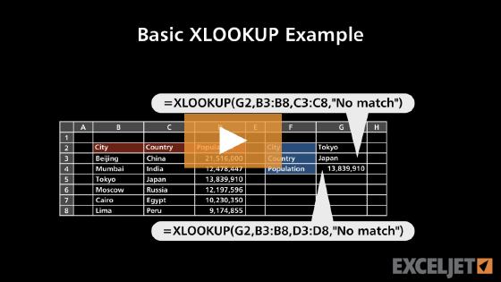
For a quick demonstration of XLOOKUP in action, watch this 3-minute video:
Video: Basic XLOOKUP example (3 minutes)
Table of Contents
- Exact match
- Approximate match
- Multiple values
- Two-way lookup
- Custom not found message
- Wildcard match
- Regex match
- Multiple criteria
- Complex multiple criteria
- Binary search
- Match mode options
- Search mode options
- Advantages of XLOOKUP
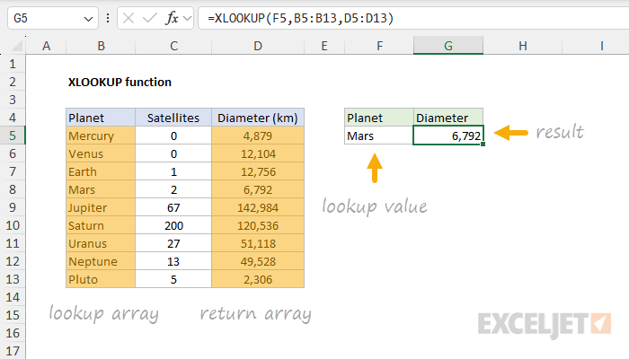
Exact match
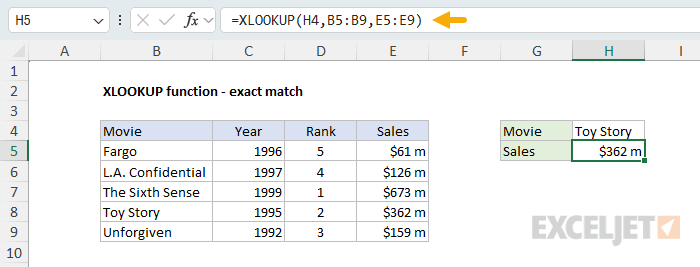
By default, XLOOKUP will perform an exact match. In the example below, XLOOKUP is configured to retrieve the Sales amount from column E based on an exact match of the movie titles in column B. The formula in H5 is:
=XLOOKUP(H4,B5:B9,E5:E9)
More detailed explanation here.
Approximate match
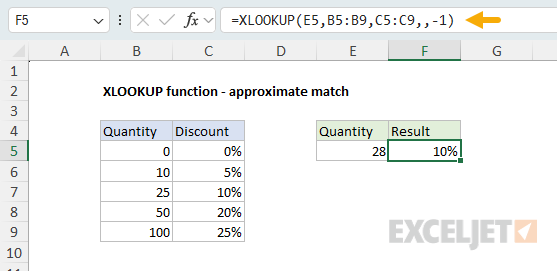
To enable an approximate match, provide a value for the match_mode argument. In the example below, XLOOKUP is used to calculate a discount based on quantity, which requires an approximate match. The formula in F5 sets match_mode to -1 to enable approximate match with "exact match or next smallest" behavior:
=XLOOKUP(E5,B5:B9,C5:C9,,-1)
More detailed explanation here.
Multiple values
XLOOKUP can return more than one value at the same time (i.e., an array of values) with one formula. The example below shows how XLOOKUP can be used to return three values with a single formula. The formula in C5 is:
=XLOOKUP(B5,B8:B15,C8:E15)
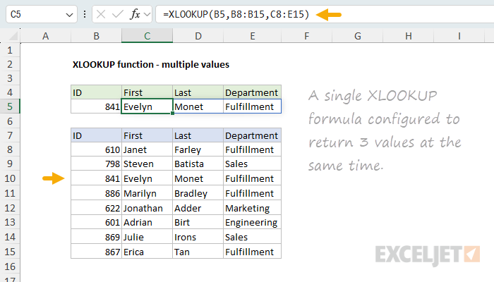
Notice the return array (C8:E15) includes 3 columns: First, Last, and Department. All three values are returned and spill into the range C5:E5.
In the example above, we use XLOOKUP to return multiple values from the same matching record. If your goal is to return more than one matching record (for example, all people in the Sales Department), XLOOKUP is not a good choice because it will return only one match. In that case, you should switch to the FILTER function, which is designed to return all matching records from a dataset based on a given set of logical conditions.
Two-way lookup
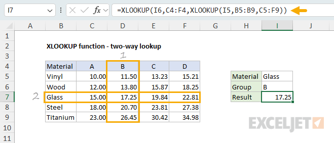
XLOOKUP can perform a two-way lookup by nesting one XLOOKUP inside another. In the example below, the "inner" XLOOKUP retrieves an entire row (all values for Glass), which is handed off to the "outer" XLOOKUP as the return array. The outer XLOOKUP finds the appropriate group (B) and returns the corresponding value (17.25) as the final result.
=XLOOKUP(I6,C4:F4,XLOOKUP(I5,B5:B9,C5:F9))
Not found message
When XLOOKUP can't find a match, it returns the #N/A error, like other match functions in Excel. Unlike the other match functions, XLOOKUP supports an optional argument called not_found that can be used to override the #N/A error when it would otherwise appear. Typical values for not_found include "Not found", "No match", "No result", etc. For example, to display "Not found" when no matching movie is found, you can use a formula like this:
=XLOOKUP(H4,B5:B9,E5:E9,"Not found")
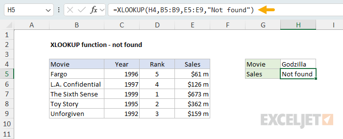
You can customize this message as you like. You can even supply an empty string ("") to display nothing when a match is not found.
Note: Be careful if you supply an empty string ("") for not_found because it hides the #N/A error that XLOOKUP will display by default. If you want to see the #N/A error when a match isn't found, omit the not_found argument entirely.
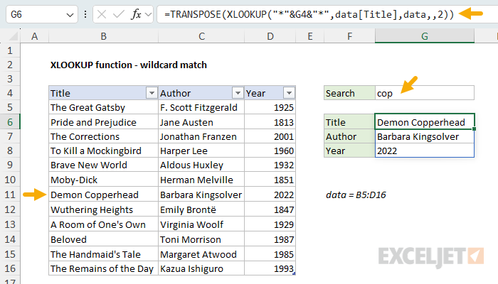
Wildcard match
XLOOKUP supports wildcards to enable partial match lookups. Set the match_mode argument to 2 to enable wildcards in XLOOKUP. In the example below, XLOOKUP is configured to perform a "contains substring" match on the Titles of the books listed in column B. The search string is entered in cell G4, and the formula in cell G6 is:
=TRANSPOSE(XLOOKUP("*"&G4&"*",data[Title],data,,2))
Read a complete explanation here. For a slightly simpler formula, see this page.
Regex match
In Excel 365, XLOOKUP can match with Regular Expressions (also called "regex"). In the worksheet below, the goal is to look up the correct price of the product number entered in cell F4 using the product codes in column B. This problem is trickier than it looks. Each product code begins with 3 uppercase letters and ends with 2 or 3 uppercase letters. In the middle of the product code is a number between 2 and 4 digits. A wildcard match won't work because a number like 56 can appear inside other product codes. However, we can easily solve this problem with a "regex match". To enable a regex match in XLOOKUP, provide 3 for match_mode. Then supply a valid regex pattern as the lookup_value. In the worksheet below, the formula in cell F5 looks like this:
=XLOOKUP("[A-Z]{3}"&F4&"[A-Z]{2,3}",B5:B16,C5:C16,,3)
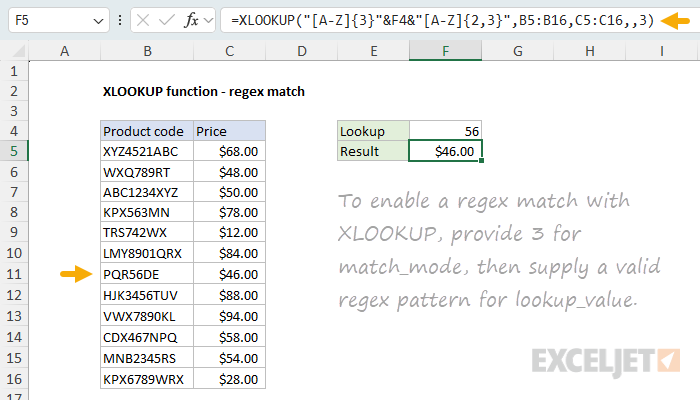
The regex pattern in this formula is "[A-Z]{3}"&F4&"[A-Z]{2,3}", which becomes [A-Z]{3}56[A-Z]{2,3}. The translation is "3 uppercase letters A-Z, followed by the value in F4 (56), followed by 2-3 uppercase letters A-Z". Regex is a powerful and somewhat complex language. For a detailed explanation of this particular example (including the workbook), see this page.
Regex is a complicated and deep topic. For an introduction to regex in Excel, see Regular Expressions in Excel. Regex support in XLOOKUP is only available in Excel 365.
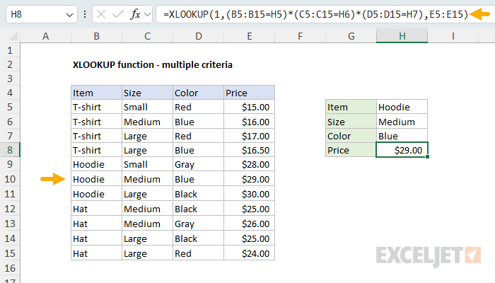
Multiple criteria
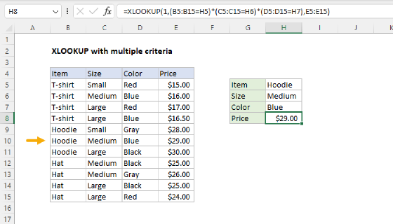
One common challenge with XLOOKUP is how to apply multiple criteria. For example, how do you look up the price for a Medium Blue Hoodie when the item, size, and color are all in different columns? A good approach is to assemble a new lookup array composed of 1s and 0s using Boolean logic and then change the lookup value to 1. This sounds complicated, but it is quite straightforward. You can see this approach in the worksheet below, where the formula in H8 looks like this:
=XLOOKUP(1,(B5:B15=H5)*(C5:C15=H6)*(D5:D15=H7),E5:E15)
Each of the three expressions generates an array of TRUE and FALSE values. The math operation (multiplication) automatically converts the TRUE and FALSE values to 1s and 0s:
{0;0;0;0;1;1;1;0;0;0;0}*{0;1;0;0;0;1;0;1;1;0;0}*{0;1;0;1;0;1;0;0;0;0;0}
After multiplication is complete, we have a single array like this:
{0;0;0;0;0;1;0;0;0;0;0}
XLOOKUP uses this array as the lookup_array. Notice the sixth value in the array is 1. This corresponds to the sixth row in the data, which contains a Medium Blue Hoodie. XLOOKUP finds the 1 and returns the corresponding value in the return_array (E5:E15), which is $29.00. For more details and to download the worksheet, see this page.
Note: Boolean logic doesn't work well for approximate match problems because it collapses the lookup array to 1s and 0s, losing the values needed for approximate matching. If you need multiple criteria with an approximate match, see this example.
Complex multiple criteria
With the ability to handle arrays natively, XLOOKUP can be used to apply complex criteria using the method explained above. In the worksheet below, XLOOKUP is configured to match the first record where (1) the account begins with "x", and (2) the region is "east", and (3) the month is not April. The formula in G5 looks like this:
=XLOOKUP(1,(LEFT(B5:B16)="x")*(C5:C16="east")*NOT(MONTH(D5:D16)=4),B5:E16)
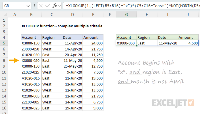
See this page for a more detailed explanation of how this formula works.
Fast binary search
XLOOKUP has a binary search mode option that performs lookups very quickly. To use binary search mode, data must be sorted in ascending or descending order. If values are sorted in ascending order, use the value 2 for search_mode. If values are sorted in descending order, use the value -2. Below is the generic syntax to enable binary search mode for an exact match lookup:
=XLOOKUP(A1,lookup_array,return_array,,0,2) // binary search A-Z
=XLOOKUP(A1,lookup_array,return_array,,0,-2) // binary search Z-A
For a more detailed example, see XLOOKUP binary search.
Match mode options
By default, XLOOKUP will perform an exact match. Match behavior is controlled by an optional argument called match_mode, which has the following options:
| Match mode | Behavior |
|---|---|
| 0 (default) | Exact match. Will return #N/A if no match. |
| -1 | Exact match or the next smaller item. |
| 1 | Exact match or the next larger item. |
| 2 | Wildcard match (*, ?, ~) |
| 3 | Regex match |
In December 2024, XLOOKUP was upgraded to allow a regex match in Excel 365. You can find a detailed example here. The XMATCH function was also updated to support regex. For more about regex in Excel, see Regular Expressions in Excel.
Search mode options
By default, XLOOKUP will start matching from the first data value. Search behavior is controlled by an optional argument called search_mode, which provides the following options:
| Search mode | Behavior |
|---|---|
| 1 (default) | Search from the first value |
| -1 | Search from the last value (reverse) |
| 2 | Binary search values sorted in ascending order |
| -2 | Binary search values sorted in descending order |
Binary searches are very fast, but data must be sorted as required. If data is not sorted properly, a binary search can return invalid results that look perfectly normal. Detailed example here.
XLOOKUP advantages
XLOOKUP offers several important advantages compared to VLOOKUP:
- XLOOKUP can look up data to the right or to the left of lookup values
- XLOOKUP defaults to an exact match
- XLOOKUP can work with vertical and horizontal data
- XLOOKUP can perform a reverse search (last to first)
- XLOOKUP can return entire rows or columns, not just one value
For a more detailed comparison, see XLOOKUP vs VLOOKUP. What about INDEX and MATCH? This is a much closer contest. For details, see XLOOKUP vs INDEX and MATCH.
Notes
- XLOOKUP can work with both vertical and horizontal arrays.
- XLOOKUP will return #N/A if the lookup value is not found.
- Like the INDEX function, XLOOKUP returns a reference as a result.
- The size of the lookup_array must be compatible with the return_array, or XLOOKUP will return #VALUE!
- If XLOOKUP points to an Excel Table in an external workbook, the other workbook must be open or XLOOKUP will return a #REF! error.