Summary
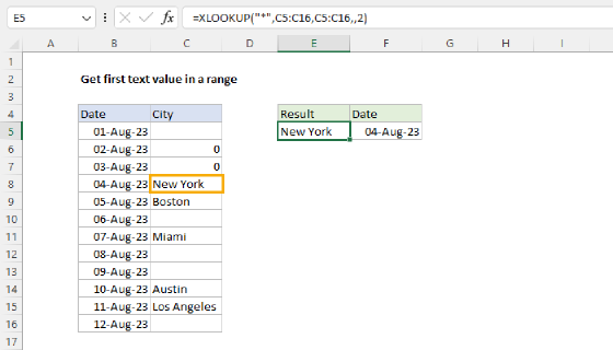
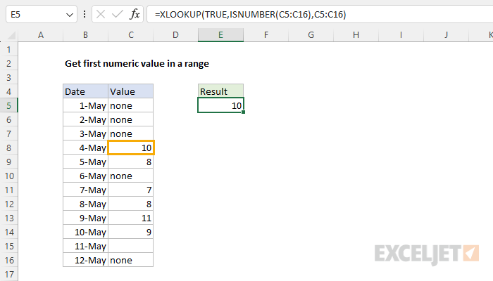
To get the first number in a row or column you can use the XLOOKUP function with the ISNUMBER function. In the example shown, the formula in E5 is:
=XLOOKUP(TRUE,ISNUMBER(C5:C16),C5:C16)
This formula finds the first numeric value in the range C5:C16, which in this case, is 10.
Generic formula
=XLOOKUP(TRUE,ISNUMBER(range),range)
Explanation
The general goal is to return the first numeric value in a row or column. More specifically, in the worksheet shown, we have dates in column B and a numeric value in the range C5:C16. Notice that all of the cells in this range have numeric values. Some are blank and some contain text values. We want the first number that appears in the range C5:C16. This problem can be solved using the XLOOKUP function or, in older versions of Excel, an INDEX and MATCH formula. Both methods are explained below.
XLOOKUP function
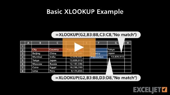
The XLOOKUP function is a modern upgrade to the VLOOKUP function. XLOOKUP is flexible and can handle many different lookup scenarios. The generic syntax for required inputs looks like this:
=XLOOKUP(lookup_value,lookup_array,return_array)
Where each argument has the following meaning:
- lookup_value - the value to look for
- lookup_array - the range or array to search within
- return_array - the range or array to return values from
For more details, see How to use the XLOOKUP function.
The ISNUMBER function
The ISNUMBER function returns TRUE when a cell contains a number, and FALSE if a cell is empty or contains a text value. If A1 contains "Age", A2 contains 32, and cell A3 is empty, the ISNUMBER function returns the following:
=ISNUMBER(A1) // returns FALSE
=ISNUMBER(A2) // returns TRUE
=ISNUMBER(A3) // returns FALSE
For more details, see How to use the ISNUMBER function.
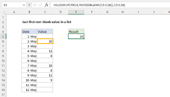
XLOOKUP formula
In the worksheet shown, the formula in cell E5 combined XLOOKUP and ISNUMBER like this:
=XLOOKUP(TRUE,ISNUMBER(C5:C16),C5:C16)
At a high level, the XLOOKUP function is configured with the lookup_value set to TRUE. The lookup_array is generated with the ISNUMBER function here:
ISNUMBER(C5:C16)
Because the range C5:C16 contains 12 cells, ISNUMBER returns an array that contains 12 TRUE and FALSE results like this:
{FALSE;FALSE;FALSE;TRUE;TRUE;FALSE;TRUE;TRUE;TRUE;TRUE;FALSE;FALSE}
The TRUE values in this array indicate cells that contain numbers. The FALSE values indicate cells that either contain text values or are empty, such as cell C16. This array is then returned directly to the XLOOKUP function as the lookup_array. At this point, we have the following:
=XLOOKUP(TRUE,{FALSE;FALSE;FALSE;TRUE;TRUE;FALSE;TRUE;TRUE;TRUE;TRUE;FALSE;FALSE},C5:C16)
With a lookup value of TRUE, XLOOKUP matches the first TRUE in the lookup_array (the fourth value), and returns the corresponding value from the range C5:C16 (10) as a final result.
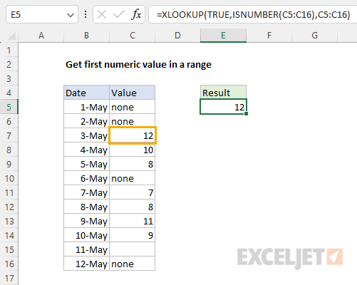
Testing the formula
This formula is dynamic and will always return the first numeric value. To test the formula, we can add the number 12 to cell C7. Now the formula returns the 12, since 12 becomes the first numeric value in the range C5:C16.
INDEX and MATCH formula
In older versions of Excel that do not provide the XLOOKUP function, you can use an array formula based on INDEX and MATCH like this:
=INDEX(C5:C16,MATCH(TRUE,ISNUMBER(C5:C16),0))
Note: this is an array formula and must be entered with control + shift + enter in Excel 2019 and older.
This formula uses the same logic as the XLOOKUP formula above. The MATCH function is used to find the position of the first numeric value in C5:C16.
MATCH(TRUE,ISNUMBER(C5:C16),0)
The ISNUMBER function returns an array of TRUE (numeric) and FALSE (not numeric) values:
{FALSE;FALSE;FALSE;TRUE;TRUE;FALSE;TRUE;TRUE;TRUE;TRUE;FALSE;FALSE}
The array is returned to the MATCH function as the lookup_array. The lookup_value is given as TRUE and match_type is set to 0 to require an exact match:
MATCH(TRUE,{FALSE;FALSE;FALSE;TRUE;TRUE;FALSE;TRUE;TRUE;TRUE;TRUE;FALSE;FALSE},0)
MATCH then returns the location of the first TRUE in the array (4) as the row number to INDEX:
=INDEX(C5:C16,4) // returns 10
INDEX then returns the value from the fourth cell in C5:C16 (10) as a final result.
For more details, see How to use INDEX and MATCH.