=INDEX(array, row_num, [col_num], [area_num])- array - A range of cells, or an array constant.
- row_num - The row position in the reference or array.
- col_num - [optional] The column position in the reference or array.
- area_num - [optional] The range in reference that should be used.
Using the INDEX function
The INDEX function returns the value at a given location in a range or array. INDEX is a powerful and versatile function. You can use INDEX to retrieve individual values or entire rows and columns. INDEX is frequently used together with the MATCH function. In this scenario, the MATCH function locates a value and feeds the numeric position to the INDEX function, and INDEX returns the value at that position.
In the most common usage, INDEX takes three arguments: array, row_num, and col_num. Array is the range or array from which to retrieve values. Row_num is the row number from which to retrieve a value, and col_num is the column number at which to retrieve a value. Col_num is optional and not needed when array is one-dimensional.
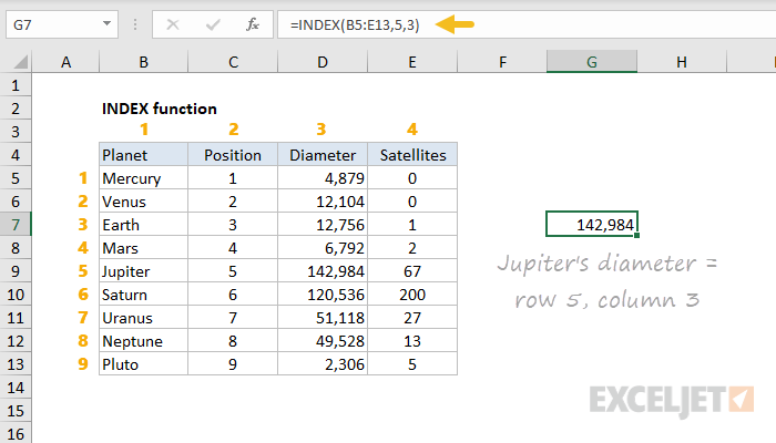
In the example shown above, the goal is to get the diameter of the planet Jupiter. Because Jupiter is the fifth planet in the list, and Diameter is the third column, the formula in G7 is:
=INDEX(B5:E13,5,3) // diameter of Jupiter
The formula above is of limited value because the row and column numbers have been hard-coded. Typically, the MATCH function would be used inside INDEX to provide these numbers. For a detailed explanation with many examples, see How to use INDEX and MATCH.
Basic usage
INDEX gets a value at a given location in a range of cells based on numeric position. When the range is one-dimensional, you only need to supply a row number. When the range is two-dimensional, you must supply both the row and column numbers. For example, to get the third item from the one-dimensional range A1:A5:
=INDEX(A1:A5,3) // returns value in A3
The formulas below show how INDEX can be used to get a value from a two-dimensional range:
=INDEX(A1:B5,2,2) // returns value in B2
=INDEX(A1:B5,3,1) // returns value in A3
INDEX and MATCH
In the examples above, the position is "hardcoded". Typically, the MATCH function is used to find positions for INDEX. For example, in the screen below, the MATCH function is used to locate "Mars" (G6) in row 3 and feed that position to INDEX. The formula in G7 is:
=INDEX(B5:E13,MATCH(G6,B5:B13,0),3)
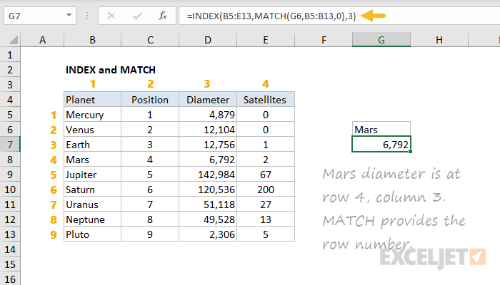
MATCH provides the row number (4) to INDEX. The column number is still hardcoded as 3.
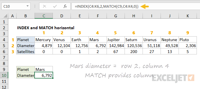
INDEX and MATCH with horizontal table
In the screen below, the table above has been transposed horizontally. The MATCH function returns the column number (4) and the row number is hardcoded as 2. The formula in C10 is:
=INDEX(C4:K6,2,MATCH(C9,C4:K4,0))
For a detailed explanation with many examples, see: How to use INDEX and MATCH
Entire row / column
INDEX can be used to return entire columns or rows like this:
=INDEX(range,0,n) // entire column
=INDEX(range,n,0) // entire row
where n represents the number of the column or row to return. This example shows a practical application of this idea.
Reference as result
It's important to note that the INDEX function returns a reference as a result. For example, in the following formula, INDEX returns A2:
=INDEX(A1:A5,2) // returns A2
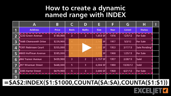
In a typical formula, you'll see the value in cell A2 as a result, so it's not obvious that INDEX is returning a reference. However, this is a useful feature in formulas like this one, which uses INDEX to create a dynamic named range. You can use the CELL function to report the reference returned by INDEX.
Two forms
The INDEX function has two forms: array and reference. Both forms have the same behavior – INDEX returns a reference in an array based on a given row and column location. The difference is that the reference form of INDEX allows more than one array, along with an optional argument to select which array should be used. Most formulas use the array form of INDEX, but both forms are discussed below.
Array form
In the array form of INDEX, the first parameter is an array, which is supplied as a range of cells or an array constant. The syntax for the array form of INDEX is:
INDEX(array,row_num,[col_num])
- If both row_num and col_num are supplied, INDEX returns the value in the cell at the intersection of row_num and col_num.
- If row_num is set to zero, INDEX returns an array of values for an entire column. To use these array values, you can enter the INDEX function as an array formula in a horizontal range, or feed the array into another function.
- If col_num is set to zero, INDEX returns an array of values for an entire row. To use these array values, you can enter the INDEX function as an array formula in a vertical range, or feed the array into another function.
Reference form
In the reference form of INDEX, the first parameter is a referenceto one or more ranges, and a fourth optional argument, area_num, is provided to select the appropriate range. The syntax for the reference form of INDEX is:
INDEX(reference,row_num,[col_num],[area_num])
Just like the array form of INDEX, the reference form of INDEX returns the reference of the cell at the intersection row_num and col_num. The difference is that the reference argument contains more than one range, and area_num selects which range should be used. The area_num is argument is supplied as a number that acts like a numeric index. The first array inside reference is 1, the second array is 2, and so on.
For example, in the formula below, area_num is supplied as 2, which refers to the range A7:C10:
=INDEX((A1:C5,A7:C10),1,3,2)
In the above formula, INDEX will return the value at row 1 and column 3 of A7:C10.
- Multiple ranges in reference are separated by commas and enclosed in parentheses.
- All ranges must on one sheet or INDEX will return a #VALUE error. Use the CHOOSE function as a workaround.