Summary
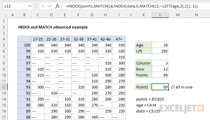
In this example, the goal is to determine the correct points to assign based on a given lift amount. Points are in column B, lift data is in columns C:I, and age is in row 4. The formula in L12 uses INDEX, MATCH, and the LEFT function:
=INDEX(points,MATCH(L6,INDEX(data,0,MATCH(L5,--LEFT(age,2),1)),-1))
where points (B5:B25), age (C4:I4), and data (C5:I25) are named ranges. The formula returns is 89 points, based on an age of 28 in L5, and a lift of 295 in L6.
Notes: this is an advanced formula. For step-by-step introduction to INDEX and MATCH, see this article. This is also an array formula that must be entered with control + shift + enter in Legacy Excel. In Excel 365, the formula does not need special handling.
Explanation
This example is based on a fitness assessment where the goal is to award points based on how much weight was lifted at a given age. The solution described below is based on an INDEX and MATCH formula, but there are several tricky elements that must be considered, making this problem much more difficult than your average lookup problem. The formula in L12 is:
=INDEX(points,MATCH(L6,INDEX(data,0,MATCH(L5,--LEFT(age,2),1)),-1))
The formulas in L8:L10 are for additional explanation only. They show how the problem can be broken down into intermediate steps.
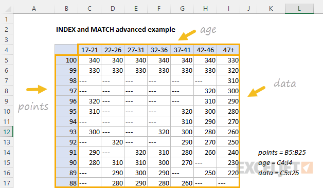
Data layout
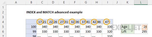
The first step is to verify the structure of the data and the behavior that will be needed to solve this problem. In column B, the range B5:B25 contains points. The formula will ultimately need to return a number from this range as the final result. In row 4, the range C4:I4 contains age ranges. Finally, the range C5:I25 contains lift data. There are three named ranges in the worksheet: points (B5:B25), age (C4:I4), and data (C5:I25). These named ranges are for convenience only, to make the formula easier to read and write.
Behavior
When a user enters an age in L5 and a lift in L6, the formula should calculate points based on these two inputs. This means the formula needs to match the correct age column, locate the best match in the lift data, then traverse back to column B to get a final result. At a high level, there are three steps:
- look up the age column
- Look up lift
- Retrieve points
The screen below shows an overview:
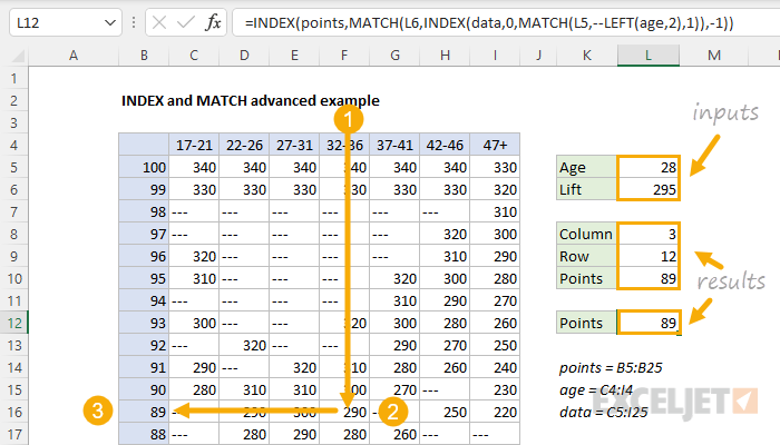
Note: the formulas in L8:L10 are just to make it easier to understand how the formula works, they are not used in the final formula in L12.
Complications
This problem is notable because the configuration is "backwards" from what is usually expected. Instead of matching an outer row and column, and retrieving a value from inside the table, we need to match a value inside the table and traverse back to an outer column (points). Also note that both the age lookup and the lift lookup are approximate match lookups, and the lift data appears in descending order. Finally, the ages in row 4 are text strings, whereas the age in L5 is numeric.
Age column
To get the correct age column we can use the MATCH function together with the LEFT function like this:
=MATCH(L5,--LEFT(age,2),1)
Working from the inside out, the first step is to identify the correct column number by matching the age in L5 against the age ranges in C4:I4. This is more difficult than usual, because while the age in L5 is a number, the age ranges in C4:I4 are text strings. Looking at the age ranges, the first thing to note is that we only need the first number in each age range to get the right match:
 '
'
We can extract just the first number of each age range with the LEFT function like this:
--LEFT(age,2)
Because we are giving MATCH a range that contains 7 values, we get back 7 results in an array like this:
{"17","22","27","32","37","42","47"}
The double negative (--) converts these text values to actual numbers, resulting in an array of numeric values:
{17,22,27,32,37,42,47}
We now have what we need to get the column number with the MATCH function. The array above as lookup_array, and with age in L5, we have:
=MATCH(L5,{17,22,27,32,37,42,47},1)
We use 1 for match_type, because we want to find the largest value that is less than or equal to age. Simplifying, we have:
=MATCH(28,{17,22,27,32,37,42,47},1) // returns 3
The MATCH function returns 3 since 27 is the correct match, and the third item in the list.
The lift
Now that we know which age column we should use to look up the lift, we can move on to that task. This too is complicated. We know the column number is 3, and we know the lift data is in data (C5:I25), but how do we look up a lift of 295 with that information? The trick is to extract just column 3 (age range 27-31) before we look up the lift. We can do that with the INDEX function like this:
=INDEX(data,0,3) // returns column 3
By providing zero for row_num and 3 for column_num, INDEX will return the entire third column of data (C5:I25), which is the range E5:E25. So, putting it all together, we have:
INDEX(data,0,MATCH(L5,--LEFT(age,2),1)) // returns E5:E25
The MATCH function returns 3 to the INDEX function as column_num, and INDEX returns column 3 of data. We now have what we need to finally look up the lift. To do this, we embed the code above into another MATCH function:
MATCH(L6,INDEX(data,0,MATCH(L5,--LEFT(age,2),1)),-1)
Note the lookup_value is the lift from cell L6 (295) and match_type is -1, since the lift data appears in descending order and we want to find the smallest value that is greater than or equal to the lift. The lookup_array is created with the code explained above. Simplifying, we have:
MATCH(295,E5:E25,-1) // returns 12
MATCH returns 12 because 300 is the smallest value that is greater than or equal to 295, the position of 300 is in row 12 of E5:E25. Just to recap, all of the code below simply returns the number 12:
MATCH(L6,INDEX(data,0,MATCH(L5,--LEFT(age,2),1)),-1) // returns 12
We now have everything we need to solve the problem. We know the correct lift is in row 12 and column 3 of data, so we just need to traverse back across row 12 to retrieve the corresponding value from points (B5:B25). How can we do that? This is actually the easiest step in the problem. All we need to do is give the INDEX function the points range with a row number:
=INDEX(points,12) // returns 89
Recap
Putting everything together, the final formula in L12 is:
=INDEX(points,MATCH(L6,INDEX(data,0,MATCH(L5,--LEFT(age,2),1)),-1))
The inner MATCH function returns 3 to the inner INDEX as column_num:
=INDEX(points,MATCH(L6,INDEX(data,0,3),-1))
With 0 for row_num, INDEX returns the range E5:E25 to the outer MATCH as lookup_array:
=INDEX(points,MATCH(L6,E5:E25,-1))
The outer MATCH returns 12 as row_num to INDEX*:*
=INDEX(points,12)
Finally, the INDEX function returns 89, the points awarded for a lift of 295 at age 28.