Summary
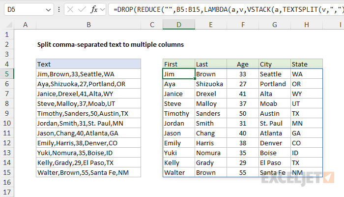
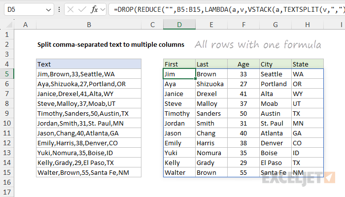
To split comma-separated values (CSV) into multiple columns with a formula, you can use the TEXTSPLIT function. In the example below, we use TEXTSPLIT together with REDUCE and VSTACK to split all comma-separated values in column B into multiple columns in one step. The formula in cell D5 looks like this:
=DROP(REDUCE("",B5:B15,LAMBDA(a,v,VSTACK(a,TEXTSPLIT(v,",")))),1)
Because there are 5 values in each row, the result is a horizontal array of separate values that spills across 5 columns in the range D5:H15. The REDUCE function is needed to allow TEXTSPLIT to process all 11 values in column B at once. See below for a much simpler formula to process one row at a time.
This is a formula-based solution. If you don't want to use a formula, you can use Excel's Text-to-Columns feature, which is a one-off manual process. If you need more automation, or are working with larger sets of data, possibily split across many files, Power Query is a better solution.
Generic formula
=TEXTSPLIT(A1,",")
Explanation
In this example, the goal is to split comma-separated values (CSV) in column B into multiple columns, as seen in the worksheet shown. Each text string in column B contains 5 fields separated by commas, so we expect to get 5 columns of data as a result. The header row in column D is manually entered.
One disadvantage of the TEXTSPLIT + REDUCE + VSTACK formula featured in this article is that it is somewhat complex. See below for a TEXTSPLIT + TEXTJOIN alternative formula that is much simpler, but note that it will fail on large sets of data.
Table of Contents
- How TEXTSPLIT works
- TEXTSPLIT to split one row
- TEXTSPLIT with REDUCE to split all rows
- TEXTSPLIT with a dynamic range
- Choose specific columns
- TEXTSPLIT with TEXTJOIN alternative
- Formula for Legacy Excel
- Extract nth field
- Text-to-columns alternative
How TEXTSPLIT works
The core of the solution is the TEXTSPLIT function, which is designed to split delimited text strings into multiple columns or rows. For example, if we give TEXTSPLIT a string like "red,blue,green", and provide a comma (",") as the column delimiter, it will return an array that contains three values:
=TEXTSPLIT("red,blue,green",",") // returns {"red","blue","green"}
Because we provided a comma (",") as the column delimiter, TEXTSPLIT splits the text string into a horizontal array of values. When this array is returned to the worksheet, it spills into multiple columns.
For more details on how TEXTSPLIT works, see our TEXTSPLIT function page.
TEXTSPLIT to split one row
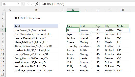
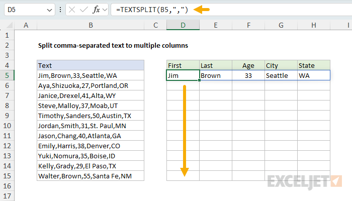
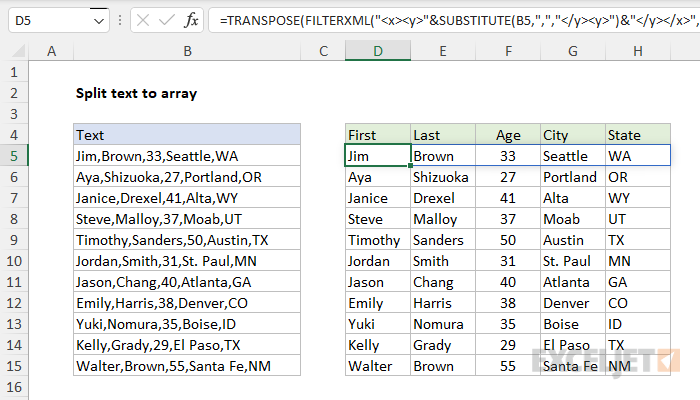
Before we look at how TEXTSPLIT can be configured to process a range of values, let's see how we can use TEXTSPLIT to split a single row of comma-separated values. In the worksheet shown, the text in cell B5 is "Jim,Brown,33,Seattle,WA". To split this text into five separate values, we can use the following formula in cell D5:
=TEXTSPLIT(B5,",")
Although TEXTSPLIT can take up to six separate arguments, in this case, we only need to provide the first two arguments, text and col_delimiter. Notice we must provide the comma as text surrounded by double quotes (","). The result is a horizontal array with five values like this:
{"Jim","Brown","33","Seattle","WA"}
This array is returned to cell D5. Because the comma has been provided as the column delimiter, the five values spill into the range D5:H5:
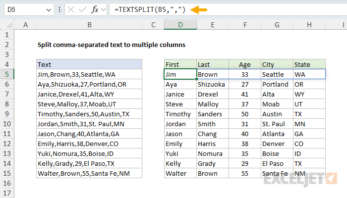
When we copy the formula down to cell D15, we have results for all 11 rows split into comma-separated values into multiple columns:
At this point, you might think we can simply give TEXTSPLIT a range of values to process all rows at the same time. Like this:
=TEXTSPLIT(B5:B15,",")
However, due to a limitation in Excel, this won't work. Excel will not allow a formula to return an array of arrays. Instead, Excel will truncate the results to the first value only:
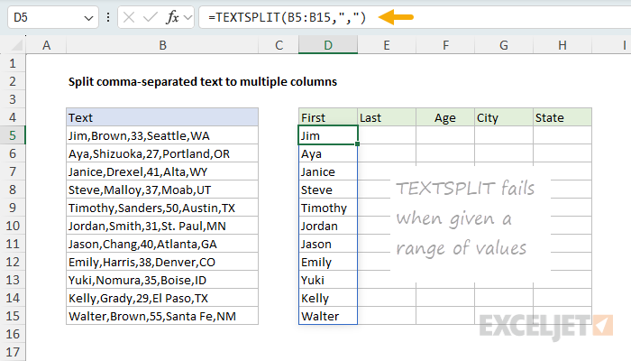
To make a formula that will process all rows at the same time, we need to upgrade the formula significantly.
There is no requirement to process all rows at the same time. Setting up the formula to handle one row at a time is much simpler, but it does require copying the formula down to each row.
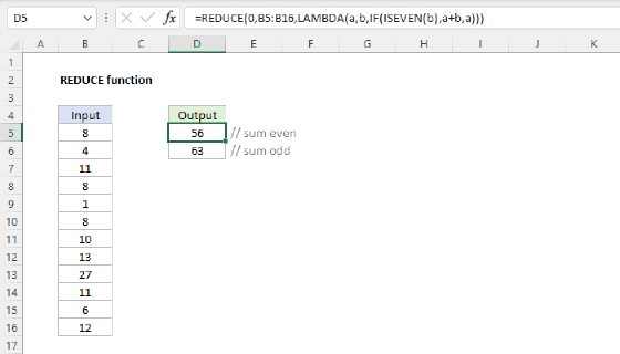
TEXTSPLIT with REDUCE to split all rows
One way to make Excel process all comma-separated values in column B at the same time is to use the REDUCE function in a formula like this:
=DROP(REDUCE("",B5:B15,LAMBDA(a,v,VSTACK(a,TEXTSPLIT(v,",")))),1)
When we enter this formula in cell D5, all results are returned in one go:
This is a pretty advanced formula, so let's work through it step-by-step. At a high level, we use the REDUCE function to loop through the text values in B5:B15 one by one. For each new value, we apply the TEXTSPLIT function to split each comma-separated value and use the VSTACK function to stack the results vertically. REDUCE works by applying a custom LAMBDA function to each value in a given array, and it accumulates results to a single value. The generic syntax looks like this:
REDUCE(initial_value,array,lambda(a,v,calculation))
The a is the accumulator (the running result), and v is each value in the array. These values are passed into the LAMBDA by REDUCE for each iteration. The actual work is done by the LAMBDA function, which is configured like this:
LAMBDA(a,v,VSTACK(a,TEXTSPLIT(v,",")))
As REDUCE loops through the range, the LAMBDA function splits each value v with TEXTSPLIT:
TEXTSPLIT(v,",") // split value by comma
And then adds the result to the accumulating results a with the VSTACK function:
VSTACK(a,TEXTSPLIT(v,",")) // stack results vertically
Because the REDUCE function has been configured to start with an empty text string (""):
REDUCE("",B5:B15,LAMBDA(...))
We will end up with an extra blank row at the top of our results. To remove this blank row, we use the DROP function:
DROP(REDUCE(...),1)
DROP removes the first row from the array returned by REDUCE. The final result is a single array that contains 11 rows, just like the source data column B. This array lands in cell D5 and spills into the range D5:H15.
The reason this formula works is that the REDUCE function returns a single array, instead of an array of arrays. The final array is built up one row at a time using the VSTACK function as REDUCE loops over the values.
TEXTSPLIT with a dynamic range
Because the REDUCE version of the formula is much more complicated than the original text split formula above, you might wonder — why bother? One answer is that this formula will work with any number of rows. In other words, you can feed a dynamic range into this formula, and the results will expand to include all values in the range. For example, we can adjust the formula to use a dynamic range by adding the TRIMRANGE function like this:
=DROP(REDUCE("",TRIMRANGE(B5:B1000),LAMBDA(a,v,VSTACK(a,TEXTSPLIT(v,",")))),1)
Or we can use the dot operator syntax like this:
=DROP(REDUCE("",B5:.B1000,LAMBDA(a,v,VSTACK(a,TEXTSPLIT(v,",")))),1)
In both cases, the range provided to reduce will expand to include new values added up to row 1000. You can see how this works below, where I have adjusted the formula to use the dot operator syntax and added a new comma-separated text value to cell B16:
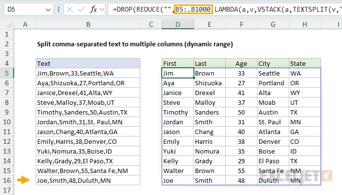
Notice the range provided to REDUCE is now B5:.B1000, which expands to include new values added up to row 1000. All empty trailing rows are automatically removed from the range before it is passed to REDUCE.
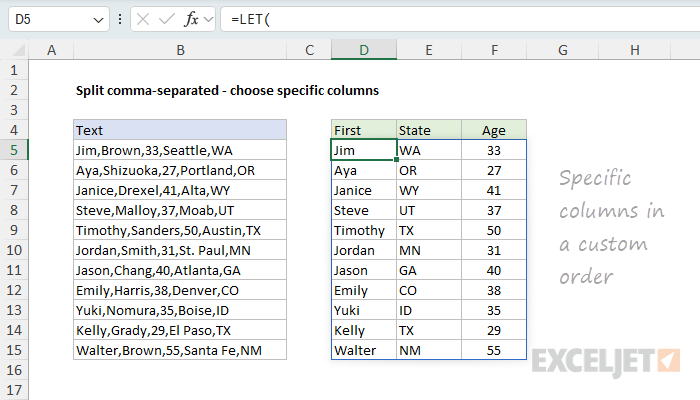
Choose specific columns
If you only want specific columns from the CSV you can easily adjust the formula to include the CHOOSECOLS function. For example, to get just the first name, state, and age, you can use a formula like this
=LET(
rng,B5:.B1000,
result,DROP(REDUCE("",rng,LAMBDA(a,v,VSTACK(a,TEXTSPLIT(v,",")))),1),
CHOOSECOLS(result,{1,5,3})
)
Here, we've adjusted the formula to use the LET function in order to define two variables: rng and result. The rng variable is the range of values to process, and result is the array of results from the REDUCE function. We then use the CHOOSECOLS function to select only columns 1, 5, and 3 from the result array. Notice we are using the dynamic range syntax explained in the previous section, so the results will expand if new values are added. Also, we have reordered the columns by passing the array {1,5,3} to CHOOSECOLS:
CHOOSECOLS(result,{1,5,3})
Here is the final result:
TEXTSPLIT with TEXTJOIN alternative
A different and simpler way to approach this problem is to use a formula based on TEXTSPLIT and TEXTJOIN:
=TEXTSPLIT(TEXTJOIN(";",,B5:B15),",",";")
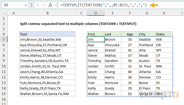
This is a clever approach that relies on TEXTSPLIT's ability to split text into rows and columns at the same time. Basically, we use the TEXTJOIN function first to concatenate all values in the range using a semicolon (";") as the delimiter. Then we feed the concatenated text into the TEXTSPLIT function, which is configured to use a comma (",") for the column delimiter and a semicolon (";") for the row delimiter. TEXTSPLIT then splits the concatenated text into rows and columns at the same time. This works great, and the formula runs quickly. However, there is an important limitation.
Excel cells have a hard limit of 32,767 characters, and if TEXTJOIN produces a result that exceeds this limit, it returns a #CALC! error, which causes the formula to fail. What this means is that if you have a lot of data, the formula may not work. At some point, as the range expands and/or the number of CSV fields increases, the character count of the concatenated text will exceed 32,767, and the formula will return an error. The TEXTSPLIT + REDUCE + VSTACK formula will continue to work on larger data sets, but it will slow down.
The bottom line? TEXTSPLIT + TEXTJOIN is a compact and elegant formula that leverages TEXTSPLIT's ability to split text into 2d arrays. It works great on smaller data sets, but it will fail on large data sets.
Formula for Legacy Excel
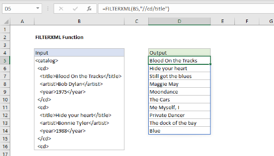
Note: Before TEXTSPLIT, you could use a hacky workaround formula based on the FILTERXML function to split comma-separated values into multiple columns. This approach doesn't make any sense to use today. However, I'm leaving it here for reference as a reminder of how complicated things used to be before the introduction of dynamic arrays, spills and TEXTSPLIT. This approach only works in Windows versions of Excel, since the Mac version of Excel does not have the FILTERXML function.
In older versions of Excel without TEXTSPLIT, you can use a more complicated formula based on the FILTERXML function with help from the SUBSTITUTE and TRANSPOSE functions. The formula looks like this:
=TRANSPOSE(FILTERXML("<x><y>"&SUBSTITUTE(B5,",","</y><y>")&"</y></x>","//y"))
To use FILTERXML, we need XML, so the first task is to add XML markup to the text. We are going to arbitrarily make each field in the text an element, enclosed with a parent element. We start with the SUBSTITUTE function here:
SUBSTITUTE(B5,",","</y><y>")
The result from SUBSTITUTE is a text string like this:
"Jim</y><y>Brown</y><y>33</y><y>Seattle</y><y>WA"
To ensure well-formed XML tags and to wrap all elements in a parent element, we prepend and append more XML tags like this:
"<x><y>"&SUBSTITUTE(B5,",","</y><y>")&"</y></x>"
This yields a text string like this (line breaks added for readability)
"<x>
<y>Jim</y>
<y>Brown</y>
<y>33</y>
<y>Seattle</y>
<y>WA</y>
</x>"
This text is delivered directly to the FILTERXML function as the xml argument, with an Xpath expression of "//y":
FILTERXML("<x><y>Jim</y><y>Brown</y><y>33</y><y>Seattle</y><y>WA</y></x>","//y")
Xpath is a parsing language and "//y" selects all elements. The result from FILTERXML is a vertical array like this:
{"Jim";"Brown";33;"Seattle";"WA"}
Because we want a horizontal array in this instance, we wrap the TRANSPOSE function around FILTERXML:
=TRANSPOSE({"Jim";"Brown";33;"Seattle";"WA"})
The result is a horizontal array like this:
{"Jim","Brown",33,"Seattle","WA"}
In older versions of Excel, you can enter this formula as a multi-cell array formula in D5:H5. In Excel 365, the array will spill into the range D5:H5 automatically.
I learned the FILTERXML trick from Bill Jelen in a MrExcel video. FILTERXML is not available in Excel on the Mac, or in Excel Online. This is a nerdy workaround for difficult problems in older versions of Excel, but it doesn't make sense in a modern version of Excel. The new TEXTSPLIT function is a much better method.
If you don't want to use FILTERXML, or can't because you are using Excel on a Mac, this example shows another way to split text with a delimiter. This approach requires a bit more setup.
Extract nth field
With either option above, you may want to extract just the nth field from a single text string. To do that, you can use the INDEX function. For example, to extract just the age with TEXTSPLIT, you can use a formula like this:
=INDEX(TEXTSPLIT(B5,","),3) // get age
Notice we have simply nested the original formula inside the INDEX function. With FILTERXML, the formula looks like this:
=INDEX(TRANSPOSE(FILTERXML("<x><y>"&SUBSTITUTE(B5,",","</y><y>")&"</y></x>","//y")),3)
Text-to-columns alternative
Formulas work great when you need a solution that is dynamic, because formulas will update automatically if data changes. However, if you only need a one-off manual process, you can also use Excel's Text-to-Columns feature.