SORTBY Function

The SORTBY function sorts the contents of a range or array based on the values from another range or array. The result is a dynamic array that will "spill" onto the worksheet. If values in the source data change, the output from SORTBY updates automatically.

The first argument, array, is the data to sort. The second argument, by_array1, contains the values used for sorting. These values can come from an existing range or from an array created by a formula — see Sort by custom list below for an example. The key feature of SORTBY is that by_array1 values do not need to be part of the source data and do not need to appear in the output. However, by_array1 must have dimensions compatible with array. The optional sort_order1 argument controls direction: 1 for ascending (default), -1 for descending. To sort by more than one level, provide additional by_array and sort_order pairs.

Excel contains two functions for sorting: SORT and SORTBY. The SORT function is the simpler option when data already contains the values needed for sorting. SORTBY handles two specific situations that SORT can't:

1. You want to sort by values that shouldn't appear in the output.
2. The values you need to sort by aren't part of your source data at all.

Use SORTBY when the values to sort by need to be calculated, or should be excluded in the output, or both. This could be to sort in a custom order, or to sort by text length, date component, or extracted substring. Also, because SORTBY references ranges directly, instead of by column index like SORT, it can handle column additions and deletions more gracefully.

Note that SORT won't automatically adjust the source range if data is added or deleted. To configure SORT with a range that automatically adjusts to fit the data, use an Excel Table or a dynamic range created with TRIMRANGE or the dot operator.

Video: Basic SORTBY function example

Key features

• Returns a dynamic array that spills automatically
• Sorts values don't need to appear in source data or output
• Auto-detects orientation from by_array (vertical = sort rows, horizontal = sort columns)
• Supports multiple sort levels (up to 64 pairs)
• More resilient to column changes than SORT (references ranges, not index numbers)
• Works with Excel Tables and structured references

Table of contents

• Basic usage
• Sort by score
• Sort horizontally
• Sort by two columns
• Sort text by length
• Sort by custom list
• Sort birthdays by month and day
• Random sort
• Sort by substring
• Related functions
• Notes

Basic usage

To sort by values in another range:

=SORTBY(B5:B16,C5:C16) // sort B by C values, ascending
=SORTBY(B5:B16,C5:C16,-1) // sort B by C values, descending

To sort by a calculated value:

=SORTBY(B5:B16,LEN(B5:B16)) // sort by text length
=SORTBY(B5:B16,RANDARRAY(12)) // random sort

To sort by multiple levels:

=SORTBY(B5:D14,D5:D14,1,C5:C14,-1) // by D ascending, then C descending

Sort by score

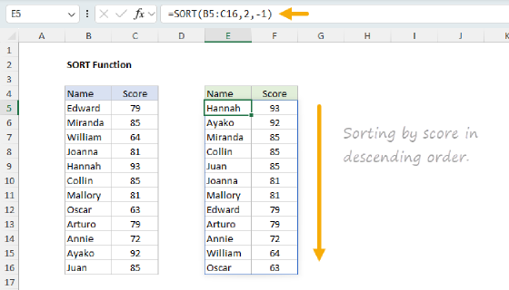
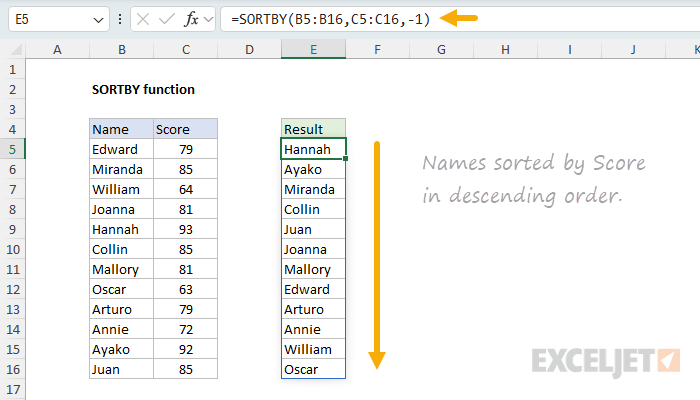
One of the key advantages of SORTBY is the ability to sort data using values that don't appear in the output. In the worksheet below, the goal is to sort the names in column B by the scores in column C, in descending order. The formula in E5 is:

=SORTBY(B5:B16,C5:C16,-1)

The array argument is B5:B16 (names only), while by_array1 is C5:C16 (scores). Because only the names are provided for array, the scores are used for sorting but don't appear in the output. The sort_order1 of -1 sorts in descending order, so the highest score appears first. To include both names and scores in the output, provide the full range as array:

=SORTBY(B5:C16,C5:C16,-1) // returns both names and scores

Sort horizontally

Unlike the SORT function, SORTBY does not have an argument that controls sorting by rows versus columns. Instead, SORTBY auto-detects the sort orientation from the shape of by_array. When by_array1 is a vertical range (one column), SORTBY sorts by row vertically. When by_array1 is a horizontal range (one row), SORTBY sorts by column horizontally. In the worksheet below, names appear in row 4 and scores in row 5, arranged horizontally. The goal is to sort by score in descending order. The formula in B8 is:

=SORTBY(B4:K5,B5:K5,-1)

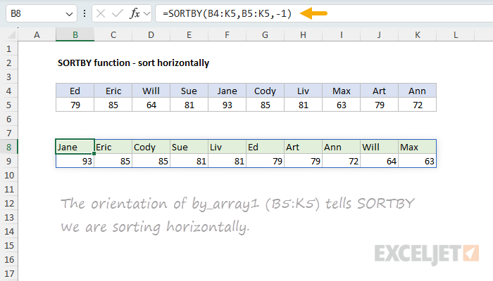
Because by_array1 (B5:K5) is a single row, SORTBY sorts by columns rather than rows. Both rows are rearranged so the highest score appears in the first column. This is different from the SORT function, which requires an explicit by_col argument set to TRUE for horizontal sorting. With SORTBY, the orientation is automatic.

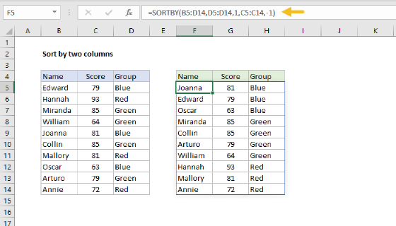
Sort by two columns

SORTBY supports multiple sort levels by providing additional by_array and sort_order pairs. In the worksheet below, the goal is to sort data first by Group in ascending order, then by Score in descending order. The formula in F5 is:

=SORTBY(B5:D16,C5:C16,1,D5:D16,-1)

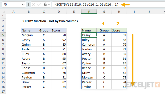
The first by_array is C5:C16 (Group) with sort_order 1 (ascending), and the second by_array is D5:D16 (Score) with sort_order -1 (descending). The result is data grouped alphabetically (A first, then B), with scores sorted from highest to lowest within each group.

For more details, see Sort by two columns.

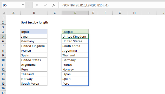
Sort text by length

SORTBY can sort data by a value calculated with a formula. In the worksheet below, the goal is to sort the country names in column B by character length, with the shortest names first. The formula in D5 is:

=SORTBY(B5:B16,LEN(B5:B16))

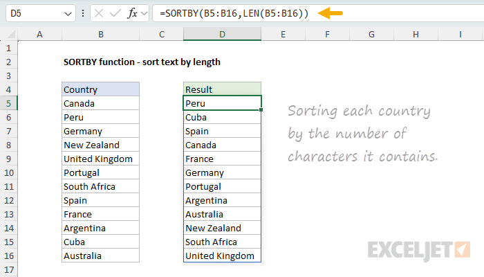
The LEN function returns an array of character counts — one for each value in B5:B16. SORTBY uses this array to sort the country names from shortest to longest. The sort values (character counts) are calculated on the fly and never appear on the worksheet.

For more details, see Sort text by length.

Sort by custom list

SORTBY is especially useful for sorting data in a custom, non-alphabetical order. In the worksheet below, the goal is to sort a table by the Priority column using the custom order in J5:J7 (High, Medium, Low). The formula in F5 is:

=SORTBY(B5:D14,MATCH(D5:D14,J5:J7,0))

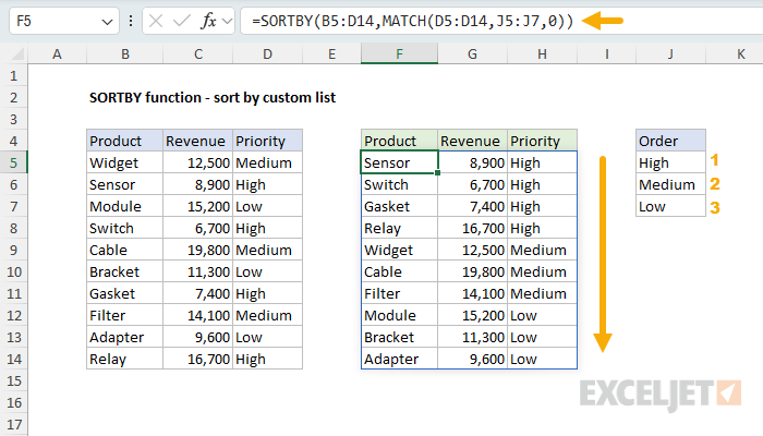
The MATCH function looks up each priority value in the custom list and returns its position: High = 1, Medium = 2, Low = 3. SORTBY uses these numeric positions to sort the data, placing High-priority items first. This approach works with any custom order — simply list the values in the desired sequence. With XMATCH, the formula is a bit shorter, since XMATCH defaults to an exact match:

=SORTBY(B5:D14,XMATCH(D5:D14,J5:J7))

For more details, see Sort by custom list.

Sort birthdays by month and day

SORTBY can sort dates by month and day while ignoring the year. In the worksheet below, the goal is to sort a list of names and birthdays in calendar order. The formula in E5 is:

=SORTBY(B5:C16,TEXT(C5:C16,"mmdd"))

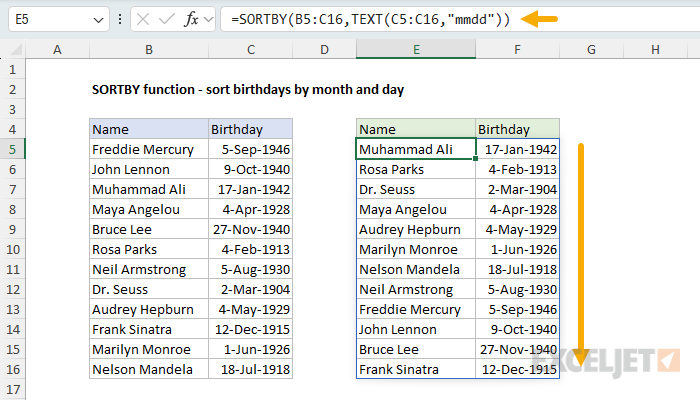
The TEXT function extracts just the month and day from each date using the format "mmdd" (e.g., July 18 becomes "0718"). SORTBY uses these text values to sort the data in calendar order, ignoring the birth year. Without this approach, sorting by date directly would sort by year first, placing the oldest people at the top.

For more details, see Sort birthdays by month and day.

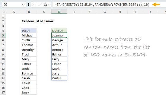
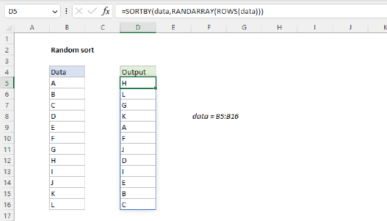
Random sort

SORTBY can randomize the order of a list when combined with the RANDARRAY function. In the worksheet below, the goal is to shuffle the values in column B into a random order. The formula in D5 is:

=SORTBY(B5:B16,RANDARRAY(ROWS(B5:B16)))

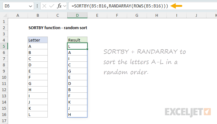
The ROWS function returns 12 (the number of rows in B5:B16), and RANDARRAY generates 12 random decimal numbers. SORTBY uses these random values to sort the data, producing a different order each time the worksheet recalculates.

RANDARRAY is a volatile function and will recalculate every time the worksheet changes. To keep a random order fixed, copy the results and use Paste Special > Values.

For more details, see Random sort.

To create random sorting that will not change and can be reproduced, see: How to do a seeded random sort in Excel.

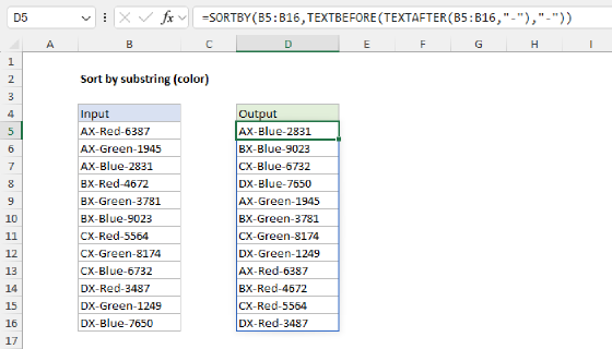
Sort by substring

SORTBY can sort data by a substring extracted with a formula. In the worksheet below, product codes contain a color between hyphens (e.g., "AX-Red-6387"). The goal is to sort the codes by color. The formula in D5 is:

=SORTBY(B5:B16,TEXTBEFORE(TEXTAFTER(B5:B16,"-"),"-"))

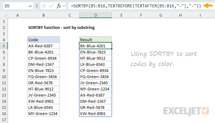
Working from the inside out, TEXTAFTER extracts everything after the first hyphen (e.g., "Red-6387"), then TEXTBEFORE extracts everything before the next hyphen (e.g., "Red"). The result is an array of color names that SORTBY uses to group the codes by color in alphabetical order.

For more details, see Sort by substring.

Notes

• SORTBY returns a #VALUE! error if by_array dimensions are not compatible with array.
• The by_array arguments must be a single row or a single column.
• The sort_order argument only accepts 1 (ascending) or -1 (descending); other values return #VALUE!.
• SORTBY returns a #SPILL! error if the output range is not empty.
• SORTBY returns a #REF! error when referencing a closed workbook (dynamic arrays require open workbooks).
• SORTBY is a "stable sort" — items with the same sort value maintain their original relative order.
• SORTBY works with Excel Tables and structured references. Results update automatically when table data changes.