Summary
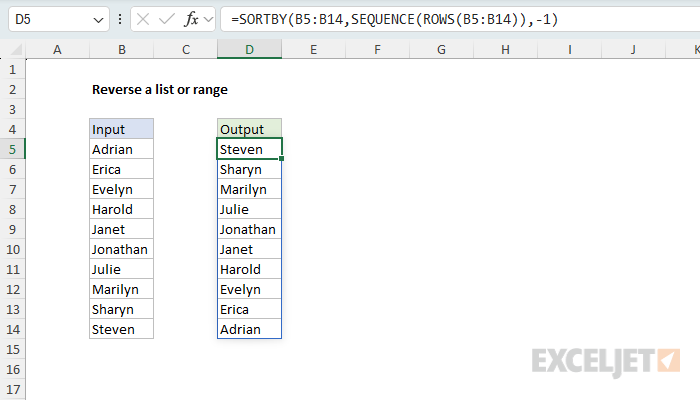
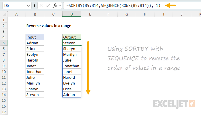
To reverse a list (i.e. arrange the values in a range in reverse order), you can use a formula based on the SORTBY function and the SEQUENCE function. In the example shown, the formula in D5, copied down, is:
=SORTBY(B5:B14,SEQUENCE(ROWS(B5:B14)),-1)
When the formula is entered in cell D5, the result is the items in the range B5:B14 sorted in reverse order: the first item appears last, the second item appears second to last, and so on.
Generic formula
=SORTBY(range,SEQUENCE(ROWS(range)),-1)
Explanation
In this example, the goal is to "reverse" the items in the range B5:B14, so that the first item appears last, the second item appears second to last, and so on. When you first encounter a problem like this in Excel, your first instinct might be to sort the values in some way using the SORT function or Excel's built-in sort feature. If the items happen to be sorted in alphabetical order, A-Z, you can indeed sort in descending order, Z-A. But what if the items are not sorted in alphabetical order? What if they are in some other order? In that case, you need to use a different approach. What we really want to do in this case is to sort the items in reverse order using their row number. The challenge is that the row number is not part of the data.
Table of contents
- Reversing values in a range
- Alternative formulas
- Reversing values in a range by columns
- Reversing a comma-separated list
- Reversing comma-separated lists for an entire range
- Reversing a range in Excel 2019 and earlier
- Implicit intersection operator
Reversing values in a range
In a current version of Excel, the easiest way to solve this problem is to use a formula based on the SORTBY function and the SEQUENCE function. This is the approach used in the worksheet shown, where the formula in D5 is:
=SORTBY(B5:B14,SEQUENCE(ROWS(B5:B14)),-1)
The SORTBY function is designed to sort an array of values in a specific order given by another array, which must be sized to match the array being sorted. In this case, the order is given by the array created by the SEQUENCE function, which is configured like this:
=SEQUENCE(ROWS(B5:B14))
Inside the SEQUENCE function, the ROWS function is used to get the number of rows in the range B5:B14. ROWS returns 10, and this is used as the rows argument in SEQUENCE. The result is an array of numbers from 1 to 10:
=SEQUENCE(ROWS(B5:B14))
=SEQUENCE(10)
={1;2;3;4;5;6;7;8;9;10}
This array is returned to SORTBY as the by_array1 argument, and sort_order1 is provided as -1, which means to sort in descending order:
=SORTBY(B5:B14,{1;2;3;4;5;6;7;8;9;10},-1)
The final result is the items in the range B5:B14 sorted in reverse order.
Another way to think of this formula is that we are first generating a set of row numbers that don't exist in the data and then using the SORTBY function to sort values in reverse order using the generated row numbers.
Pro tip: You can shorten the formula above a bit by negating the output from SEQUENCE directly, like this:
=SORTBY(B5:B14,-SEQUENCE(ROWS(B5:B14))). The output from SEQUENCE is then the negative sequence{-1;-2;-3;-4;-5;-6;-7;-8;-9;-10}and there is no need to ask SORTBY to sort in descending order. It's clever, but less intuitive for normal users.
Alternative formulas
Here are some notes on other related formulas suggested by readers. First, since we already have row numbers, why don't we use them directly like this:
=SORTBY(B5:B14,ROW(B5:B14),-1)
Here, we use the ROW function instead of the ROWS function. For the range B5:B14, ROW returns the array {5;6;7;8;9;10;11;12;13;14} and the formula works as expected. However, one key limitation of this approach is that it won't work if the input is an array; the formula needs actual row numbers. This means you can't use it to reverse an array created by another formula directly.
Jeet suggested a clever formula based on INDEX and SEQUENCE. In this formula, we get a row count with ROWS, then use SEQUENCE to build a sequence in reversed order {10;9;8;7;6;5;4;3;2;1} by starting SEQUENCE at the count c and using -1 as the step. Then we use INDEX to pick out the values at those locations:
=LET(r,B5:B14,c,ROWS(r),INDEX(r,SEQUENCE(c,1,c,-1)))
Finally, Matt Hanchett suggested a formula based on the REDUCE function:
=REDUCE(,B5:B14,LAMBDA(a,v,VSTACK(v,a)))
In this formula, we omit the initial_value to keep the formula short. This relies on an interesting behavior of REDUCE when the initial_value argument is omitted: it will use the first value in the array as the starting value of the accumulator (a). This behavior is undocumented, but mentioned here. Note that it will only work with 1D arrays. However, it's still a great example of how the REDUCE+VSTACK technique works.
Reverse values in a range by columns
To reverse the values in a range by columns, you can use a variation of the formula above. The formula in D5 looks like this:
=SORTBY(B5:K5,SEQUENCE(,COLUMNS(B5:K5)),-1)
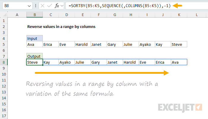
This formula is very similar to the original formula above. The difference is that we have replaced the ROWS function with the COLUMNS function , and we have added a comma to the SEQUENCE function to skip the rows argument so that SEQUENCE creates a horizontal array of numbers in columns. The result is the values in the range B5:K5 sorted in reverse order by columns.
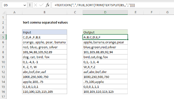
Reversing a comma-separated list
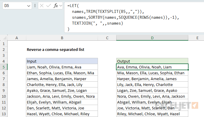
An interesting variant of the formula above is when you want to reverse the order of comma-separated values in text strings, as seen below. The gist of this solution is to use the TEXTSPLIT function to split the values into an array. Then use the formula above to sort the array in reverse order. Then use the TEXTJOIN function to join the values together again. The formula in D5 looks like this:
=LET(
  names,TRIM(TEXTSPLIT(B5,,",")),
  snames,SORTBY(names,SEQUENCE(ROWS(names)),-1),
  TEXTJOIN(", ",,snames)
)
At the highest level, the LET function is used to assign names to intermediate results. The name names is assigned the result of the TEXTSPLIT function, and the name snames is assigned the result of the SORTBY function. The TEXTJOIN function is used to join the values together again, with a comma and a space between each value. Here's how this formula works step-by-step, working from the inside out:
- The TEXTSPLIT function is used to split the values in the text string in B5 into an array of values. Notice we have skipped the col_delimiter argument, and provided a comma as the row_delimiter so that the resulting array is a single column of rows.
- The TRIM function is used to remove any leading or trailing spaces from each value. This is a normalization step to ensure that the values do not contain any leading or trailing spaces.
- The SORTBY function is used to sort the array of values in reverse order, as explained in the original formula above.
- The TEXTJOIN function is used to join the values together again, with a comma and a space between each value.
When the formula is entered in cell D5, the result is the values in the text string in B5 reversed in order. As the formula is copied down column D, the process repeats for each text string in the range B5:B14.
Notice the way we use the SORTBY function in this formula is essentially the same as the original formula above: We are sorting rows in reverse order using an array created by the SEQUENCE function.
Reversing comma-separated lists for an entire range
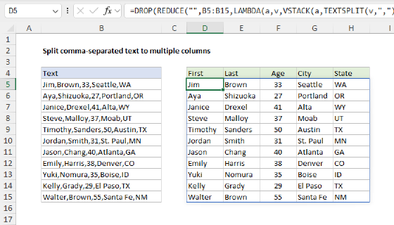
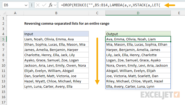
To process the entire range in one step, you can adapt the formula above to use the REDUCE function with the VSTACK function. The formula in D5 looks like this:
=DROP(REDUCE("",B5:B14,LAMBDA(a,v,VSTACK(a,LET(
  names,TRIM(TEXTSPLIT(v,,",")),
  snames,SORTBY(names,SEQUENCE(ROWS(names)),-1),
  TEXTJOIN(", ",,snames)
)))),1)
This formula works by iterating over each value in the range B5:B14 using the REDUCE function. For each value v in the range, the LAMBDA function:
- Splits the comma-separated values using TEXTSPLIT
- Trims any leading or trailing spaces using TRIM
- Reverses the order using SORTBY and SEQUENCE (as explained in the previous section)
- Joins the reversed values back together using TEXTJOIN
The VSTACK function stacks each processed result vertically into a single array. The initial value of an empty string ("") is provided to REDUCE, which creates an extra row that we remove using the DROP function. The final result is an array of reversed comma-separated lists that spills into the range D5:D14.
This pattern of using REDUCE with VSTACK is useful when you need to process each element in a range and return an array of results. The REDUCE function iterates over the range, and VSTACK progressively builds up the final array. For more examples of this pattern, see the REDUCE function page.
Reversing a range in Excel 2019 and earlier
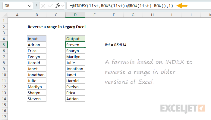
If you are using a legacy version of Excel, you can use a more complex formula based on the INDEX, ROWS, and ROW functions. The formula in D5 looks like this:
=INDEX(list,ROWS(list)+ROW(list)-ROW(),1)
This formula only makes sense if you are using an older version of Excel that does not have the SORTBY and SEQUENCE functions.
As this formula is copied down, it returns the items in reverse order. The name "list" is a named range B5:B14. Named ranges are absolute references by default, so they are convenient to use in a situation like this. If you don't use a named range, use an absolute reference like $B$5:$B$14 instead.
The heart of this formula is the INDEX function, which is given the list as the array argument:
=INDEX(list,
The second part of the formula is an expression that works out the correct row number as the formula is copied down:
ROWS(list)+ROW(list)-ROW()
- ROWS(list) returns the number of rows in the list (10 in the example)
- ROW(list) returns the first row number of
list(5 in the example) - ROW() returns the row number the formula resides in
The result of this expression is a single number starting at 10, and ending at 1 as the formula is copied down. The first formula returns the 10th item in the list, the second formula returns the 9th item in the list, and so on:
=INDEX(list,10+5-5,1) // item 10
=INDEX(list,10+5-6,1) // item 9
=INDEX(list,10+5-7,1) // item 8
etc.
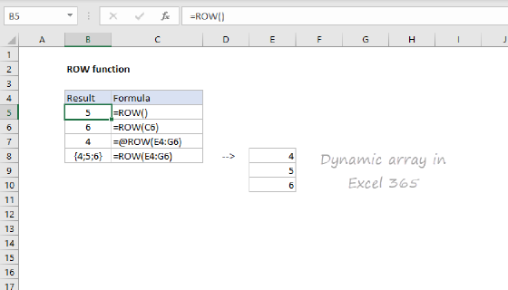
Implicit intersection operator
Note that if you enter or open the legacy formula above in a modern version of Excel, Excel will add the implicit intersection operator to the formula, as seen in the screenshot above
=@INDEX(list,ROWS(list)+@ROW(list)-ROW(),1)
This @ symbol is called the implicit intersection operator, and it disables the automatic array behavior where multiple values spill onto the worksheet. In other words, it tells Excel you want a single value. This is done to ensure that older formulas continue to return the same (single) result when they might otherwise spill multiple values onto the worksheet and generate #SPILL! errors.