Return array with INDEX function

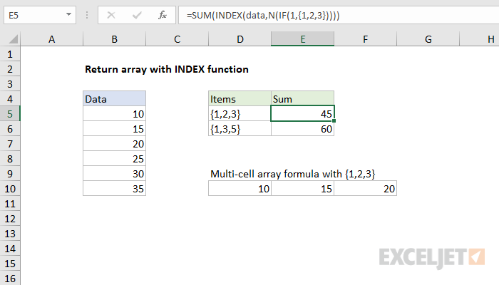
To get INDEX to return an array of items to another function, you can use an obscure trick based on the IF and N functions. In the example shown, the formula in E5 is:

=SUM(INDEX(data,N(IF(1,{1,2,3}))))

where "data" is the named range B5:B10.

In Excel 2021 and later, this trick is not necessary, thanks to dynamic arrays. See the TAKE function.

Explanation

It is surprisingly tricky to get INDEX to return more than one value to another function. To illustrate, the following formula can be used to return the first three items in the named range "data", when entered as a multi-cell array formula.

{=INDEX(data,{1,2,3})}

The results can be seen in the range D10:F10, which correctly contains 10, 15, and 20. However, if we wrap the formula in the SUM function:

=SUM(INDEX(data,{1,2,3}))

The final result is 10, while it should be 45, even if entered as an array formula. The problem is that INDEX only returns the first item in the array to the SUM function. To force INDEX to return multiple items to SUM, you can wrap the array constant in the N and IF functions like this:

=SUM(INDEX(data,N(IF(1,{1,2,3}))))

which returns a correct result of 45. Similarly, this formula:

=SUM(INDEX(data,N(IF(1,{1,3,5}))))

correctly returns 60, the sum of 10, 20, and 30.

This obscure technique is sometimes called "dereferencing", because it stops INDEX from handling results as cell references, and subsequently dropping all but the first item in the array. Instead, INDEX delivers a full array of values to SUM. Jeff Weir has a good explanation here on stackoverflow.