Sort by substring

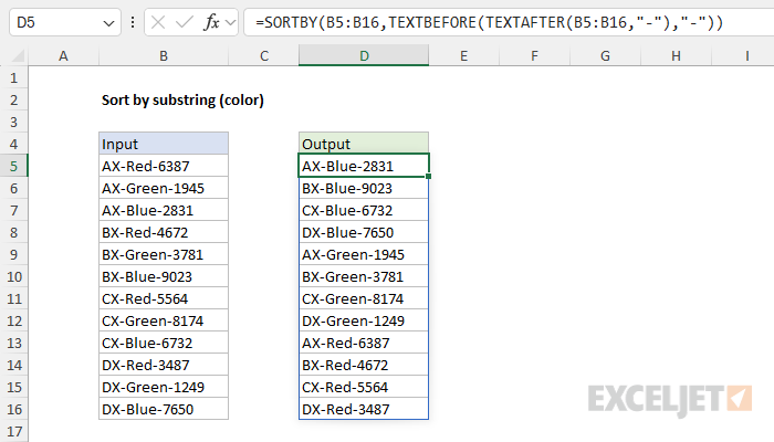
To sort data by a substring, you can use the SORTBY function together with the TEXTBEFORE and TEXTAFTER functions. In the worksheet shown, we are sorting the codes in column B by color. The formula in cell D5 is:

=SORTBY(B5:B16,TEXTBEFORE(TEXTAFTER(B5:B16,"-"),"-"))

The result in column D is a list of the same codes sorted by color in alphabetical order.

Explanation

We have a list of 12 codes in Column B. Each code consists of a prefix (two letters), a color (variable), and a 4-digit number, all separated by hyphens (e.g., AX-Red-6387). The goal is to sort this list based on the color substring so that all codes with the same color are grouped together in the output in alphabetical order. The 2-letter prefix and 4-digit number should be ignored during sorting. This is a good example of a situation where the SORTBY function is necessary instead of the standard SORT function. The formula in cell D5 looks like this:

=SORTBY(B5:B16,TEXTBEFORE(TEXTAFTER(B5:B16,"-"),"-"))

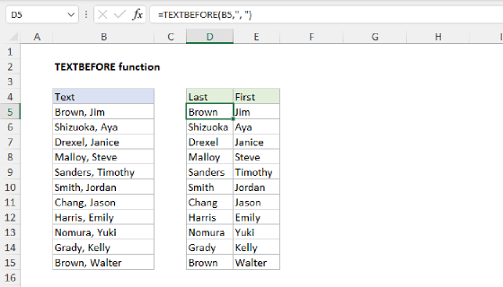
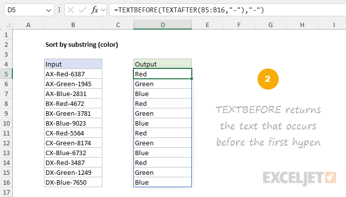
Working from the inside out, the first step is to isolate the color from the rest of the code. To do this, we use a combination of the TEXTAFTER function and the TEXTBEFORE function. First, TEXTAFTER is used to extract text that appears after the first hyphen:

TEXTAFTER(B5:B16,"-")

You can see the result in the screen below:

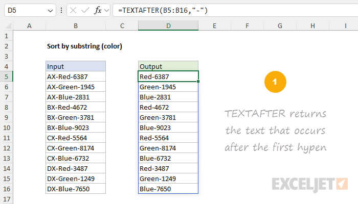
Using TEXTAFTER to extract text after the first hyphen

The result from TEXTAFTER is delivered directly to the TEXTBEFORE function:

=TEXTBEFORE(TEXTAFTER(B5:B16,"-"),"-")

The TEXTBEFORE function then extracts just the text that occurs before the first hyphen. This can be a bit confusing. The main thing to keep in mind is that TEXTBEFORE is working with the output from TEXTAFTER. This means there is only one hyphen at this point (see the screen above) since TEXTAFTER has already removed the other hyphen. The screen below shows the result after TEXTBEFORE runs:

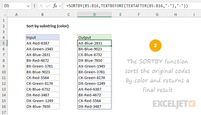
Using TEXTAFTER to isolate the color

At this point, we have isolated and extracted the color for each code. The final step is to use the colors to sort the original codes, which is done with the SORTBY function, which is the outermost function:

=SORTBY(B5:B16,TEXTBEFORE(TEXTAFTER(B5:B16,"-"),"-"))

SORTBY is configured to sort the range B5:B16 using the colors returned by TEXTBEFORE and TEXTAFTER. The final result looks like this:

SORTBY sorts the codes by the color substring

Sort by state

There are many other practical cases where the approach described above can be adapted to sort data by a substring. For example, the worksheet below shows how you can sort data in the form "City, State ZIP" by State:

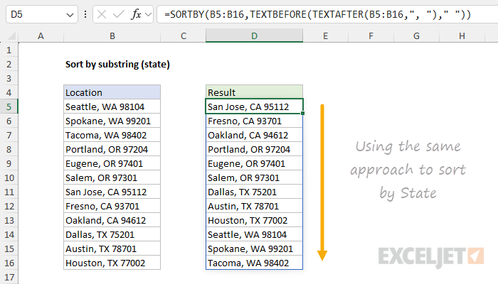
Using the same approach to sort location data by state

The formula in cell D5 is very similar to the original formula above. The difference is that the delimiters have been adjusted to match the data:

=SORTBY(B5:B16,TEXTBEFORE(TEXTAFTER(B5:B16,", ")," "))

Sort by state and city

Since SORTBY supports sorting by more than one value, we can extend the formula above to sort by State, and then by City. The result looks like this:

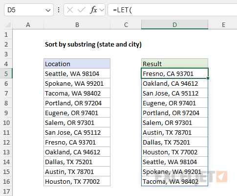
Extending the formula to sort by state and then by city

In this version, we've incorporated the LET function to keep things streamlined. The formula in cell D5 looks like this:

=LET(
data,B5:B16,
states,TEXTBEFORE(TEXTAFTER(data,", ")," "),
cities,TEXTBEFORE(data,","),
SORTBY(data,states,1,cities,1)
)

This is how the formula works:

Open with the LET function so that we can use variables.
Declare a variable named "data" and assign the range B5:B16 as the value.
Declare a variable named "states" and use TEXTBEFORE and TEXTAFTER to extract just the state abbreviations.
Declare a variable named "cities" and use TEXTBEFORE to extract just the city names.
Use the SORTBY function to sort data by states and then by cities.

This is a nice example of how the LET function can organize a more complex formula in a way that makes it easier to read and understand.