=XMATCH(lookup_value, lookup_array, [match_mode], [search_mode])- lookup_value - The lookup value.
- lookup_array - The array or range to search.
- match_mode - [optional] 0 = exact match (default), -1 = exact match or next smallest, 1 = exact match or next larger, 2 = wildcard match, 3 = regex match.
- search_mode - [optional] 1 = search from first (default), -1 = search from last, 2 = binary search ascending, -2 = binary search descending.
Using the XMATCH function
XMATCH is a modern replacement for the MATCH function. It is a flexible and versatile function with a number of useful features:
- The ability to look up values in vertical or horizontal ranges.
- Exact matching plus "next larger" and "next smaller" approximate matching.
- Simple "contains" type matching with native Excel wildcards (* ? ~).
- Complex pattern matching with "regex", a powerful text-matching language.
- A reverse search option to find the last matching value in a range.
- A super-fast binary search option when working with large datasets.
The XMATCH function performs a lookup and returns the numeric position of the lookup value as a result. XMATCH takes four arguments, and the generic syntax looks like this:
=XMATCH(lookup_value,lookup_array,[match_mode],[search_mode])
Lookup_value is the value to look for, and lookup_array is the range or array to look in. The match_mode argument controls what kind of match is performed (exact, next smallest, next largest, or wildcard). Search_mode controls the search direction (first to last or last to first) and enables the binary search option, which is optimized for speed. See below for more details.
Example
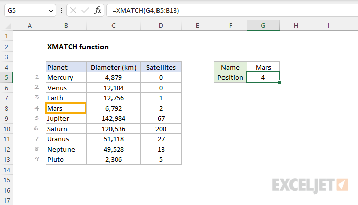
To perform an ordinary exact match, only the first two arguments are required. For example, to locate the position of the planet Mars in the worksheet shown, you can use XMATCH like this:
=XMATCH(G4,B5:B13) // returns 4
The result is 4 since "Mars" appears in the fourth row of the range B5:B13. Typically, the XMATCH function is used together with the INDEX function to retrieve a value at a specific location. For example, to find the diameter of Mars, you can combine INDEX and XMATCH like this:
=INDEX(C5:C13,XMATCH(G4,B5:B13)) // returns 6792
In this formula, XMATCH returns the position of Mars (4) to INDEX, and INDEX returns the 4th value in the range C5:C13 (6,792) as the final result.
XMATCH defaults to an exact match, so match_mode is not required above.
XMATCH vs. MATCH
XMATCH is an upgraded replacement for the MATCH function. Like the MATCH function, XMATCH performs a lookup and returns a numeric position. Also, like MATCH, XMATCH can perform lookups in vertical or horizontal ranges, supports both approximate and exact matches, and allows wildcards (* ?) for partial matches. The 5 key differences between XMATCH and MATCH are:
- XMATCH defaults to an exact match, while MATCH defaults to an approximate match.
- XMATCH can find the next larger item or the next smaller item.
- XMATCH can perform a reverse search (i.e. search from last to first).
- XMATCH does not require values to be sorted when performing an approximate match.
- XMATCH can perform a binary search, which is specifically optimized for speed.
- XMATCH can use regex for matching, a powerful pattern-matching language.
In an INDEX and MATCH formula, using XMATCH instead of the MATCH function "upgrades" the formula to include the benefits listed above.
Replacing MATCH with XMATCH
In some cases, XMATCH can be a drop-in replacement for the MATCH function. For example, for exact matches, the syntax is identical:
=MATCH(value,array,0) // exact match
=XMATCH(value,array,0) // exact match
However, for approximate matches, the behavior is different when match_type is set to 1:
=MATCH(value,array,1) // exact match or next smallest
=XMATCH(value,array,1) // exact match or next *largest*
In addition, XMATCH allows -1 for match type, which is not available with MATCH:
=XMATCH(value,array,-1) // exact match or next smallest
There are subtle differences in the behavior of MATCH and XMATCH in specific cases. For example, if cell A1 is empty, and the lookup array contains an empty cell, =XMATCH(A1, array) will return the position of the empty cell, whereas =MATCH(A1, array) will return #N/A. Let me know if you notice other differences and I will include them on this page.
Match mode
The match_mode argument controls what kind of match is performed (exact, next smallest, next largest, wildcard, or regex). Note that match_mode is an optional argument. If you do not provide a value, XMATCH will default to an exact match. The table below shows the values you can use to set match_mode:
| Match mode | Behavior |
|---|---|
| 0 (default) | Exact match. |
| -1 | Exact match or next smaller item. |
| 1 | Exact match or next larger item. |
| 2 | Wildcard match (*, ?, ~) |
| 3 | Regex match |
In December 2024, XMATCH was upgraded to allow a regex match in Excel 365. The XLOOKUP function was also updated to support regex. For more about regex in Excel, see Regular Expressions in Excel.
Search mode
The fourth argument for XMATCH is search_mode. This is an optional argument that controls search behavior as follows:
| Search mode | Behavior |
|---|---|
| 1 (default) | Search from the first value to the last |
| -1 | Search from the last value to the first (reverse) |
| 2 | Binary search values sorted in ascending order (very fast) |
| -2 | Binary search values sorted in descending order (very fast) |
Binary searches are very fast, but take care data is sorted as required. If data is not sorted properly, a binary search can return invalid results that look perfectly normal.
Exact match
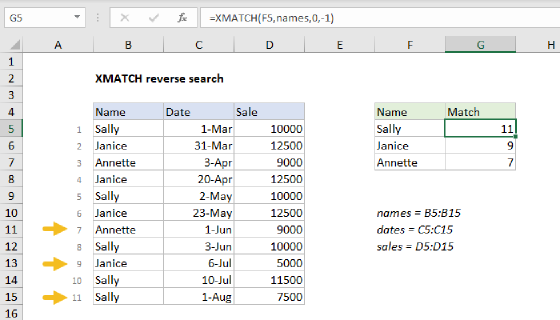
In the worksheet below, XMATCH is used to get the position of "Mars" in a list of planets in the range B6:B13. The formula in G6 is:
=XMATCH(G4,B5:B13) // returns 4
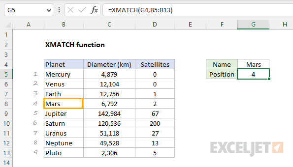
XMATCH defaults to an exact match, so there is no need to enable this behavior.
Match mode behavior
The example below illustrates match mode behavior with a lookup value of 3.1 and lookup values in B5:B11:
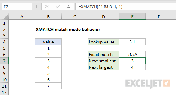
E6=XMATCH(E4,B5:B11) // returns #N/A
E7=XMATCH(E4,B5:B11,-1) // returns 3
E8=XMATCH(E4,B5:B11,1) // returns 4
- In cell E6, match_mode defaults to 0 (exact match) so the result is #N/A (not found).
- In cell E7, match_mode is given as -1 (next smallest) so the result is 3.
- In cell E8, match_mode is given as 1 (next largest) so the result is 4.
INDEX and XMATCH
XMATCH can be used just like MATCH in a normal INDEX and MATCH formula. To retrieve the diameter of Mars based on the original example above, the formula is:
=INDEX(C6:C14,XMATCH(G5,B6:B14)) // returns 6792
For more information, see How to use INDEX and MATCH.
XMATCH with wildcard
When match_mode is set to 2, XMATCH can perform a match using wildcards. In the example shown below, the formula in E5 is:
=XMATCH(E4,B5:B13,2) // returns 6
This is equivalent to:
=XMATCH("pq*",B5:B13,2)
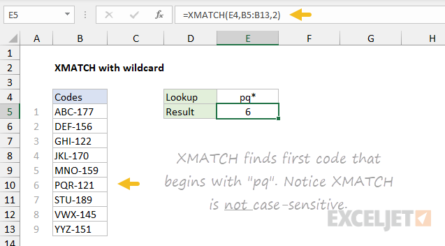
XMATCH locates the first code that begins with "pq" and returns 6 since PQR-121 appears in row 6 of the range B5:B13. Notice that XMATCH is not case-sensitive.
XMATCH with Regex
XMATCH can also match with "regex" (short for Regular Expressions). In the worksheet below, the goal is to look up the correct price of the product number entered in cell F4 using the product codes in column B. This problem is trickier than it looks. Each product code begins with 3 uppercase letters and ends with 2 or 3 uppercase letters. In the middle of the product code is a number between 2 and 4 digits. A wildcard match won't work because a number like 56 can appear inside other product codes. However, we can easily solve this problem with a "regex match". To enable a regex match in XMATCH, provide 3 for match_mode. Then supply a valid regex pattern as the lookup_value. In the worksheet below, the formula in cell F5 looks like this:
=XMATCH("[A-Z]{3}"&F4&"[A-Z]{2,3}",B5:B16,3)
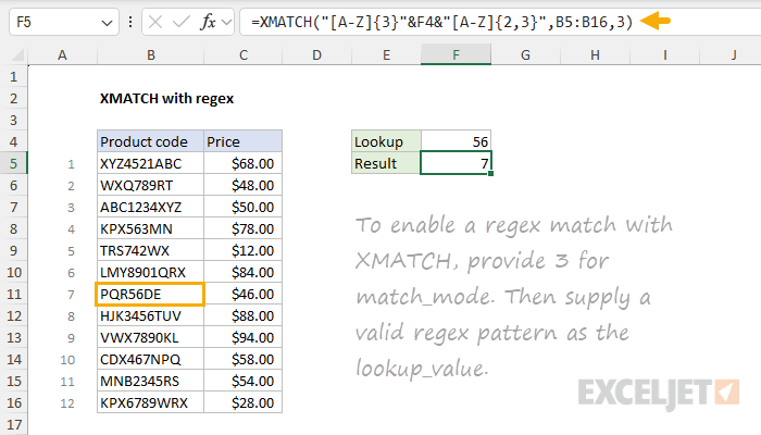
The regex pattern in this formula is "[A-Z]{3}"&F4&"[A-Z]{2,3}". The translation is "3 uppercase letters A-Z, followed by the value in F4 (56), followed by 2-3 uppercase letters A-Z". Regex is a powerful and somewhat complex language. For a detailed explanation of the regex used in this example, see XLOOKUP with regex. XLOOKUP and XMATCH support regex in the same way. Although the functions are different, the regex pattern is exactly the same.
Regex matching was added to XMATCH in December 2024, so this feature is only available in Excel 365. For an introduction to regex in Excel, see Regular Expressions in Excel.
Multiple criteria
There is no built-in way to provide multiple criteria with XMATCH but you can use Boolean logic to apply multiple conditions. In the worksheet below, XMATCH is configured to apply 3 separate conditions to match the values for Item, Size, and Color entered in H5:H7.
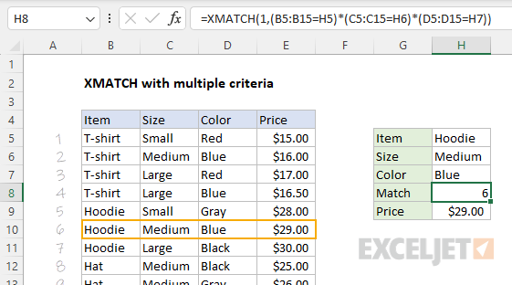
For more details, see this page.
Case-sensitive match
The MATCH function is not case-sensitive. However, MATCH can be configured to perform a case-sensitive match when combined with the EXACT function in a generic formula like this:
=XMATCH(TRUE,EXACT(lookup_value,array),0))
The EXACT function compares every value in array with the lookup_value in a case-sensitive manner. This formula is explained in an INDEX and MATCH example here. The example uses the MATCH function, but XMATCH can be substituted with the same result.
Binary search
XMATCH has a binary search option that runs very quickly. To enable binary search mode, data must be sorted in ascending or descending order. If values are sorted in ascending order, use the value 2 for search_mode. If values are sorted in descending order, use the value -2. Below is the generic syntax to enable binary search mode for an exact match lookup:
=XMATCH(value,array,0,2) // binary search A-Z
=XMATCH(value,array,0,-2) // binary search Z-A
For a more detailed example, see this page. The primary example is based on the XLOOKUP function but the explanation shows how to use INDEX and XMATCH to solve the same problem.
Notes
- XMATCH can work with both vertical and horizontal arrays.
- XMATCH will return #N/A if the lookup value is not found.
- XMATCH defaults to an exact match, while MATCH defaults to an approximate match.
- XMATCH can find the next larger item or the next smaller item.
- XMATCH can perform a reverse search (i.e. search from last to first).
- XMATCH does not require values to be sorted when performing an approximate match.
- XMATCH can perform a binary search, which is specifically optimized for speed.