Summary
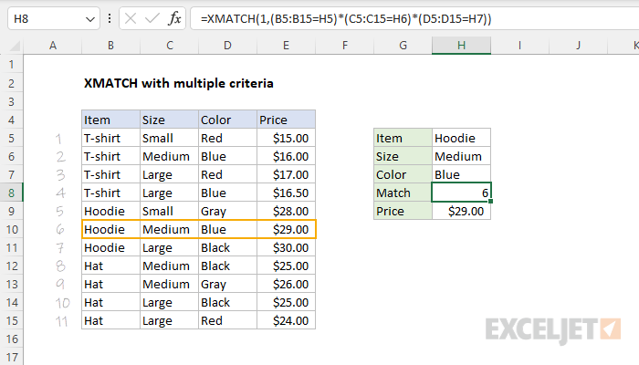
The best way to use XMATCH with multiple criteria is to use Boolean logic to apply conditions. In the example shown, the formula in H8 is:
=XMATCH(1,(B5:B15=H5)*(C5:C15=H6)*(D5:D15=H7))
The result is 6, since the sixth row in the data contains a Medium Blue Hoodie. Note the lookup_value in XMATCH is 1. This is because the lookup_array is an array that contains only 1s and 0s. Read below for details.
Generic formula
=XMATCH(1,(criteria1)*(criteria2)*(criteria3))
Explanation
The goal is to match a row in a set of data based on a given Item, Size, and Color. At a glance, this seems like a difficult problem because XMATCH only has one value for lookup_value and lookup_array. How can we configure XMATCH to consider values from multiple columns? The trick is to generate the lookup array we need using Boolean logic, then configure XMATCH to look for the number 1. This approach is explained below.
The XMATCH function
The XMATCH function is an upgraded replacement for the older MATCH function. At the core, XMATCH performs a lookup and returns the numeric position of the lookup value in a range or array as the result. XMATCH performs an exact match by default and in its simplest form, requires just two arguments, a lookup value and a lookup array:
=XMATCH(lookup_value,lookup_array)
Looking at the generic syntax above, you can see there is no obvious way to provide multiple criteria.
Boolean Logic
This formula works around this limitation by using Boolean logic to create a temporary array of ones and zeros to represent rows matching all 3 criteria, then asking XMATCH to find the first 1 in the array. The temporary array of ones and zeros is generated like this:
(B5:B15=H5)*(C5:C15=H6)*(D5:D15=H7)
This code compares the Item entered in H5 with all items, the Size in H6 with all sizes, and the Color in H7 with all colors. Each expression generates an array of TRUE and FALSE values as seen below:
{FALSE;FALSE;FALSE;FALSE;TRUE;TRUE;TRUE;FALSE;FALSE;FALSE;FALSE}*{FALSE;TRUE;FALSE;FALSE;FALSE;TRUE;FALSE;TRUE;TRUE;FALSE;FALSE}*{FALSE;TRUE;FALSE;TRUE;FALSE;TRUE;FALSE;FALSE;FALSE;FALSE;FALSE}
Tip: use F9 to see these results. Just select an expression in the formula bar, and press F9.
Next, the math operation (multiplication) automatically converts the TRUE and FALSE values to 1s and 0s:
{0;0;0;0;1;1;1;0;0;0;0}*{0;1;0;0;0;1;0;1;1;0;0}*{0;1;0;1;0;1;0;0;0;0;0}
This behavior is a basic feature of how Excel works with Boolean values. After the arrays are multiplied together, we have just a single array of 1s and 0s like this:
{0;0;0;0;0;1;0;0;0;0;0}
Notice the 6th value in the array is 1. This represents the one row in the data that meets all three conditions, since this row contains a Medium Blue Hoodie. This is the array used inside XMATCH as the lookup_array. Because the lookup_array contains only 1s and 0s, we provide 1 as the lookup_value. At this point, we can rewrite the formula like this:
=XMATCH(1,{0;0;0;0;0;1;0;0;0;0;0}) // returns 6
XMATCH matches the 1 in the sixth row of the array and returns 6 as a final result.
Visualizing arrays
The arrays explained above can be challenging to understand since they aren't visible when the formula calculates. The screen below shows how the arrays can be visualized with simple formulas in a worksheet. Columns B, C, and D correspond to the data in the example when the logical expressions for "Hoodie", "Medium", and "Blue" are being evaluated." Column F is the result of multiplying the ranges together:
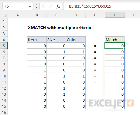
The result in F5:F15 represents the array delivered to XMATCH as the lookup_array.
INDEX and XMATCH
Typically, the XMATCH function is used in an INDEX and MATCH formula to return a value instead of a position. In the original worksheet above, the formula in cell H9 uses INDEX with XMATCH to retrieve the correct price for a Medium Blue Hoodie:
=INDEX(E5:E15,XMATCH(1,(B5:B15=H5)*(C5:C15=H6)*(D5:D15=H7)))
Notes
- The XLOOKUP function can also be configured to use multiple criteria in the same way.
- This approach can be adapted to apply more complex criteria.