Summary
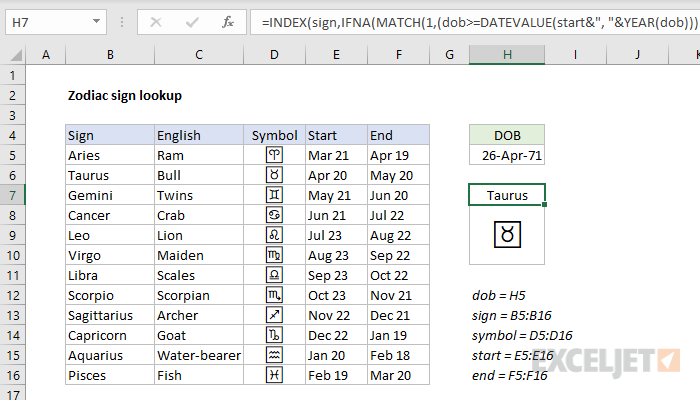
To look up one of the 12 Western Zodiac signs based on a birthdate, you can use a formula based on INDEX and MATCH. The formula in H7 is:
=INDEX(sign,IFNA(MATCH(1,(dob>=DATEVALUE(start&", "&YEAR(dob)))*(dob<=DATEVALUE(end&", "&YEAR(dob))),0),10))
where dob (H5), sign (B5:B16), symbol (D5:D16), start (E5:E15), and end (F5:F16) are named ranges. Using the lookup table as shown is somewhat challenging. See below for an alternative self-contained formula.
Explanation
The goal of this example is to look up the correct astrological or zodiac sign for a given birthdate, using the table shown in B5:F15. These are based on the Western zodiac signs described here. Zodiac signs are used in horoscopes, which are a kind of forecast of a person's future, based on the relative positions of the stars and planets at the time of birth.
Using the lookup table as shown is somewhat challenging. This article describes two ways to solve the problem. The first way uses INDEX and MATCH with the table as shown. The second way is a VLOOKUP formula with a hard-coded array constant.
Preface
For this example, I was determined to use a formula to look up a zodiac sign in an existing table (as shown) that lists each zodiac sign along with a symbol, start, and end dates. This is a challenging problem for a couple of reasons. First, the start and end dates are not actual dates, but are instead "date fragments." Second, because the zodiac signs start in March and cross over a year boundary, they are not listed in chronological order. If they were real dates in chronological order, we could use a standard INDEX and MATCH formula set up for an approximate match on the start date only. Instead, we need to configure MATCH with Boolean logic to look and locate dates that fall between two dates. In addition, we need to assemble the date fragments into actual dates, using the year from the given birthdate.
This approach works for all zodiac signs except one, Capricorn, which crosses the "new year" boundary, and means that the "between" logic will fail and never return TRUE. We could easily solve this problem by splitting the Capricorn entry into two rows with separate date ranges – one from December 22 to December 31; one for January 1 to January 19. But I didn't want to do that, since it would mess up the clean, "human-readable" lookup table.
I tried a number of tricky options to work around this problem, including shifting all dates back three months so that they fit into one year. But the complexity of these approaches bothered me (and made the formula more opaque), so in the end, I cheated by catching the #N/A error returned by MATCH in the Capricorn date range, and returning row 10, hardcoded. In other words, if a date throws an error, it must be Capricorn.
This should work fine when a valid birthdate is provided. But it also means that any invalid date will also return Capricorn – if your birthday is "apple," you are Capricorn :) Further down, I explain a sane alternative that doesn't use the table as shown.
The hard way - INDEX and MATCH with table as shown
The goal is to look up the correct zodiac sign for a given birthdate using the existing table as shown (B5:B16). The worksheet includes several named ranges for convenience: dob (H5), sign (B5:B16), symbol (D5:D16), start (E5:E15), and end (F5:F16). The formula in H7 is:
=INDEX(sign,IFNA(MATCH(1,(dob>=DATEVALUE(start&", "&YEAR(dob)))*(dob<=DATEVALUE(end&", "&YEAR(dob))),0),10))
At the core, this is a pretty standard INDEX and MATCH formula, where the MATCH function is configured to look for a "1" and the array is constructed with Boolean logic. Taking out that logic, we have:
=INDEX(sign,IFNA(MATCH(1,array,0),10))
The tricky part is in constructing the array, which is done with this expression:
(dob>=DATEVALUE(start&", "&YEAR(dob)))*(dob<=DATEVALUE(end&", "&YEAR(dob)))
On the left, we check for a dob (date of birth) greater than or equal to the start:
(dob>=DATEVALUE(start&", "&YEAR(dob))) // check start
On the right, we check for a dob less than or equal to end:
(dob<=DATEVALUE(end&", "&YEAR(dob)) // check end
The two expressions are joined with the multiplication operator (*), since multiplication corresponds with AND logic in Boolean algebra.
Inside each expression, we concatenate a date fragment from the table with the year from the birthdate, extracted with the YEAR function. Then we pass the result into the DATEVALUE function to get a valid Excel date. Because the named ranges "start" and "end" contain multiple values, the expressions above generate multiple results. With April 26, 1971 as the date of birth in H5, we get:
(dob>={26013;26043;26074;26105;26137;26168;26199;26229;26259;26289;25953;25983})*(dob<={26042;26073;26104;26136;26167;26198;26228;26258;26288;25952;25982;26012})
Then:
({TRUE;TRUE;FALSE;FALSE;FALSE;FALSE;FALSE;FALSE;FALSE;FALSE;TRUE;TRUE})*({FALSE;TRUE;TRUE;TRUE;TRUE;TRUE;TRUE;TRUE;TRUE;FALSE;FALSE;FALSE})
Then:
{0;1;0;0;0;0;0;0;0;0;0;0}
We can now simplify the original formula to:
=INDEX(sign,IFNA(MATCH(1,{0;1;0;0;0;0;0;0;0;0;0;0},0),10))
The MATCH function then returns "2" and, since "2" is not an error, we have:
=INDEX(sign,2) // returns Taurus
And the INDEX function returns the second item in sign: "Taurus" as a final result. In the event that the birthdate falls between December 22 and January 19, the "between two dates" logic will fail and MATCH will throw a #N/A error. The IFNA function will catch this error and return "10," and INDEX will return "Capricorn," the tenth item in sign (B5:B16).
As an alternative, the IFNA function or IFERROR function could be used at the outer level of the formula as well. However, I wanted the two formulas (see symbol lookup below) to be identical, except for the lookup array passed into INDEX, and I also wanted to retrieve the actual values in the table for Capricorn.
Retrieving the symbol
The formula in H8 to retrieve the symbol from the named range symbol (D5:D16), is almost identical to the original formula. The only difference is the array provided to INDEX, which is symbol instead of sign:
=INDEX(symbol,IFNA(MATCH(1,(dob>=DATEVALUE(start&", "&YEAR(dob)))*(dob<=DATEVALUE(end&", "&YEAR(dob))),0),10))
The symbols in the table are created with the UNICHAR function, introduced in Excel 2013. They start at 9800, and end at 9811:
=UNICHAR(9800) // Aries
=UNICHAR(9811) // Pisces
In Excel 365, you can generate all symbols at once using the SEQUENCE function like this:
=UNICHAR(SEQUENCE(12,1,9800)) // all 12 symbols
An easier way - VLOOKUP with an embedded table
The INDEX and MATCH formula above is based on a requirement to use the lookup table in B5:B16 as shown. If you don't need or want to show the lookup table, and if you don't mind a lookup table with two entries for Capricorn, you can use a formula based on the VLOOKUP function:
=VLOOKUP(--TEXT(dob,"m.dd"),{1.01,"Capricorn";1.2,"Aquarius";2.19,"Pisces";3.21,"Aries";4.2,"Taurus";5.21,"Gemini";6.21,"Cancer";7.23,"Leo";8.23,"Virgo";9.23,"Libra";10.23,"Scorpio";11.22,"Sagittarius";12.22,"Capricorn"},2,1)
At the core, this is a straightforward VLOOKUP formula:
=VLOOKUP(--TEXT(dob,"m.dd"),table_array,2,1)
where the table_array argument is supplied as a hard-coded array constant. If we put these values into cells, we have a table like this:
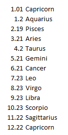
Note that the values in the first column are actual decimal numbers. Also note that Capricorn appears twice, and entries are in ascending order.
To look up a birthdate, we need a similar number, and for that, we use the TEXT function like this:
--TEXT(dob,"m.dd") // returns 4.26
Text pulls the "month" number and "day" number out of the date as text. The double negative (--) then coerces the text to a number in the same format as the lookup table above. The result for April 26, 1971 is 4.26.
Note: I ran into this approach in a post on the MrExcel board, by the always amazing Aladin Akyurek.