=SUMPRODUCT(array1, [array2], ...)- array1 - The first array or range to multiply, then add.
- array2 - [optional] The second array or range to multiply, then add.
Using the SUMPRODUCT function
The SUMPRODUCT function multiplies arrays together and returns the sum of products. If only one array is supplied, SUMPRODUCT will simply sum the items in the array. Up to 30 ranges or arrays can be supplied. When you first encounter SUMPRODUCT, it may seem boring, complex, and even pointless. But SUMPRODUCT is an amazingly versatile function with many uses. Because it will handle arrays gracefully, you can use it to process ranges of cells in clever, elegant ways.
Key features
- Works with arrays natively in older versions of Excel (no need for Ctrl+Shift+Enter)
- Can apply complex AND/OR logic using Boolean algebra
- Works for conditional sums, counts, and averages (can replace SUMIFS, COUNTIFS, AVERAGEIFS)
- Automatically treats non-numeric values as zeros (like the SUM function)
- Can use other functions like LEN, ISBLANK, ISTEXT, ISERROR, etc., directly
- Works in all Excel versions
Table of contents
- Classic SUMPRODUCT example
- SUMPRODUCT for conditional sums
- SUMPRODUCT for conditional sums and counts
- SUMPRODUCT with double negative (--)
- SUMPRODUCT with OR logic
- SUMPRODUCT with abbreviated syntax
- Ignoring empty cells
- SUMPRODUCT with other functions
- Arrays and Excel 365
Classic SUMPRODUCT example
The "classic" SUMPRODUCT example illustrates how you can calculate a sum directly without a helper column. For example, in the worksheet below, you can use SUMPRODUCT to get the total of all numbers in column F without using column F at all:
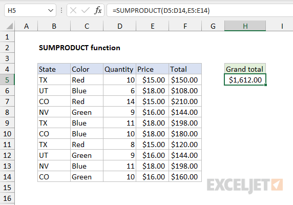
To perform this calculation, SUMPRODUCT uses values in columns D and E directly like this:
=SUMPRODUCT(D5:D14,E5:E14) // returns 1612
The result is the same as summing all values in column F. The formula is evaluated like this:
=SUMPRODUCT(D5:D14,E5:E14)
=SUMPRODUCT({10;6;14;9;11;10;8;9;11;10},{15;18;15;16;18;18;15;16;18;16})
=SUMPRODUCT({150;108;210;144;198;180;120;144;198;160})
=1612
This use of SUMPRODUCT can be handy, especially when there is no room (or need) for a helper column with an intermediate calculation. However, the most common use of SUMPRODUCT in the real world is to apply conditional logic in situations that require more flexibility than functions like SUMIFS and COUNTIFS can offer.
SUMPRODUCT for conditional sums
A typical use for the SUMPRODUCT function is to calculate conditional sums, much like you would use a function like SUMIFS. In the worksheet shown below, SUMPRODUCT is used to calculate conditional sums with four separate formulas:
=SUMPRODUCT(--(C5:C14="red"),F5:F14) // red
=SUMPRODUCT(--(B5:B14="tx"),--(C5:C14="red"),F5:F14) // tx and red
=SUMPRODUCT(--(B5:B14="co"),--(C5:C14="blue"),F5:F14) // co and blue
=SUMPRODUCT(--(C5:C14<>"red"),F5:F14) // not red
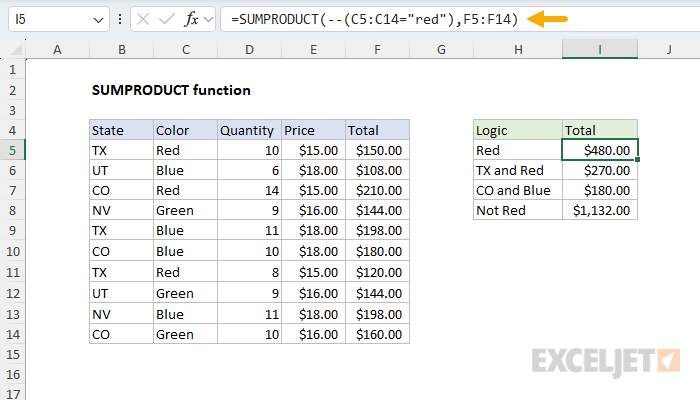
The results are visible in cells I5, I6, I7, and I8. The article below explains how SUMPRODUCT can be used to calculate these kinds of conditional sums, and the purpose of the double negative (--) in the formulas.
SUMPRODUCT for conditional sums and counts
The SUMPRODUCT function can be used for conditional sums or counts. To illustrate how this works, let's look at a very simple example. Assume we have some order data in A2:B6, with State in column A, and Sales in column B:
| A | B | |
|---|---|---|
| 1 | State | Sales |
| 2 | UT | 75 |
| 3 | CO | 100 |
| 4 | TX | 125 |
| 5 | CO | 125 |
| 6 | TX | 150 |
Using SUMPRODUCT, you can sum total sales for Texas ("TX") with this formula:
=SUMPRODUCT(--(A2:A6="TX"),B2:B6)
You can also count total sales for Texas ("TX") with this formula:
=SUMPRODUCT(--(A2:A6="TX"))
Notice we have retained the conditional logic --(A2:A6="TX") from the formula above, and simply removed the second array (Sales). This is the basic idea of counting with SUMPRODUCT. The conditional logic remains, but the second array is removed. However, to make this work, we need a way to coerce the true and false values that the logic creates into ones and zeros. Let's look at that next.
SUMPRODUCT with double negative (--)
The formulas above use a double negative (--) to make the conditional logic work properly. To understand why this is necessary, let's trace through exactly what happens when SUMPRODUCT processes our Texas example. When Excel evaluates the expression A2:A6="TX", it creates an array of TRUE and FALSE values based on which cells match "TX". Here's what the two arrays look like initially:
| array1 | array2 | Product | Result |
|---|---|---|---|
| FALSE | 75 | FALSE * 75 | 0 |
| FALSE | 100 | FALSE * 100 | 0 |
| TRUE | 125 | TRUE * 125 | 0 |
| FALSE | 125 | FALSE * 125 | 0 |
| TRUE | 150 | TRUE * 150 | 0 |
| Sum | 0 |
Array1 contains the TRUE/FALSE results from our condition, while array2 contains the corresponding sales values. The problem is that SUMPRODUCT needs to multiply these arrays together, but the raw TRUE and FALSE values can't be used directly because they are treated as zeros, making our entire calculation return zero.
This is where the double negative becomes important. The double negative is one of several ways to convert TRUE and FALSE values into their numeric equivalents: TRUE becomes 1, and FALSE becomes 0. This conversion enables Boolean logic operations within our formula. After applying the double negative, here's how the table above works:
| array1 | array2 | Product | ||
|---|---|---|---|---|
| 0 | * | 75 | = | 0 |
| 0 | * | 100 | = | 0 |
| 1 | * | 125 | = | 125 |
| 0 | * | 125 | = | 0 |
| 1 | * | 150 | = | 150 |
| Sum | 275 |
Now SUMPRODUCT can perform the calculation successfully. In array terms, the formula evaluates like this:
=SUMPRODUCT({0,0,1,0,1},{75,100,125,125,150})
SUMPRODUCT multiplies the corresponding elements of both arrays, then sums the result:
=SUMPRODUCT({0,0,125,0,150}) // returns 275
The same double negative principle applies to our conditional count example. Recall that we can count Texas sales using =SUMPRODUCT(--(A2:A6="TX")). After applying the double negative, we get the array {0,0,1,0,1}. Since we're only providing one array to SUMPRODUCT (no second array to multiply against), SUMPRODUCT simply sums the values in this single array: 0+0+1+0+1 = 2. This gives us a count of 2, representing the two rows where the state equals "TX". The double negative is essential here because without it, SUMPRODUCT would receive {FALSE,FALSE,TRUE,FALSE,TRUE} and treat these logical values as zeros, returning 0 instead of the correct count.
This example expands on the ideas above with more detail.
SUMPRODUCT with OR logic
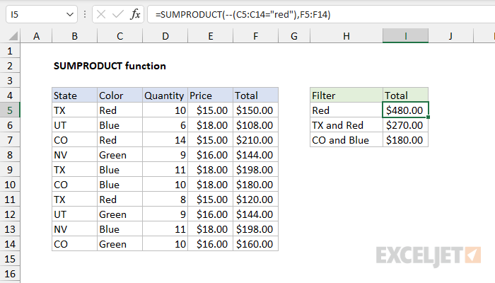
It is also possible to use the SUMPRODUCT function with OR logic, i.e., sum if this or that. The trick is to use Boolean logic, where OR logic is represented with addition (+). You can see this approach in the worksheet below:
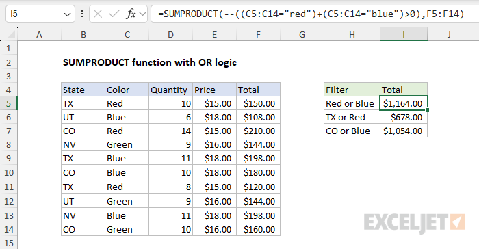
The formulas in I5:I7 are as follows:
=SUMPRODUCT(--((C5:C14="red")+(C5:C14="blue")>0),F5:F14) // red or blue
=SUMPRODUCT(--((B5:B14="tx")+(C5:C14="red")>0),F5:F14) // tx or red
=SUMPRODUCT(--((B5:B14="co")+(C5:C14="blue")>0),F5:F14) // co or blue
Notice that the two logical expressions are joined with addition (+), and the resulting array is checked against zero (>0) and then converted to 1s and 0s with the double negative (--):
--((C5:C14="red")+(C5:C14="blue")>0)
For a more detailed explanation of how and why this works, watch this 3-minute video: Boolean algebra in Excel. Also, see this example, which explains several ways to approach a problem like this.
SUMPRODUCT with abbreviated syntax
You will often see the formula described above written in a different way, like this:
=SUMPRODUCT((A2:A6="TX")*B2:B6) // returns 275
Notice that all calculations have been moved into array1. The result is the same, but this syntax provides several advantages. First, the formula is more compact, especially as the logic becomes more complex. This is because the double negative (--) is no longer needed to convert TRUE and FALSE values — the math operation of multiplication () automatically converts the TRUE and FALSE values from (A2:A6="TX") to 1s and 0s. But the most important advantage is flexibility*. When using separate arguments, the operation is always multiplication, since SUMPRODUCT returns the sum of* products*. This limits the formula to AND logic since multiplication corresponds to addition in Boolean algebra. Moving calculations into one argument means you can use addition (+) for OR logic, in any combination. In other words, you can choose your own math operations, which ultimately dictate the logic of the formula. See example here.
Even though the double negative is no longer needed, there is no harm in leaving it in the formula.
With the above advantages in mind, there is one disadvantage to the abbreviated syntax. SUMPRODUCT is programmed to ignore the errors that result from multiplying text values in arrays given as separate arguments. This can be handy in certain situations. With the abbreviated syntax, this advantage goes away, since the multiplication happens inside a single array argument. In this case, the normal behavior applies: text values will create #VALUE! errors.
Note: Technically, moving calculations into array1 creates an "array operation", and SUMPRODUCT is one of only a few functions that can handle an array operation natively without Control + Shift + Enter in Legacy Excel. See Why SUMPRODUCT? for more details.
Ignoring empty cells
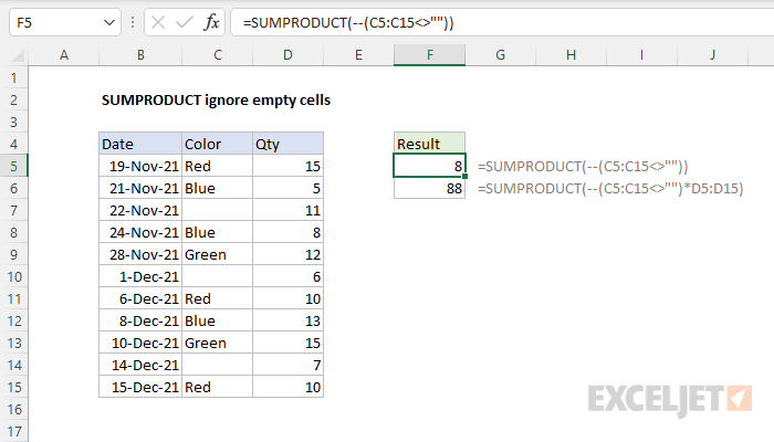
To ignore empty cells with SUMPRODUCT, you can use an expression like range<>"". In the example below, the formulas in F5 and F6 both ignore cells in column C that do not contain a value:
=SUMPRODUCT(--(C5:C15<>"")) // count
=SUMPRODUCT(--(C5:C15<>"")*D5:D15) // sum
SUMPRODUCT with other functions
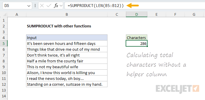
SUMPRODUCT can use other functions directly. You might see SUMPRODUCT used with the LEN function to count total characters in a range, or with functions like ISBLANK, ISTEXT, etc., to count blanks in a range or text values in a range. These are not normally array functions, but when they are given a range, they create an array of results. Because SUMPRODUCT is built to work with arrays, it is able to perform calculations on the arrays directly. You can see an example of this in the worksheet below, where we have eight text strings in the range B5:B12, and we are using SUMPRODUCT with the LEN function to calculate the total characters in the range with this formula in cell D5:
=SUMPRODUCT(LEN(B5:B12))
For example, assume you have 10 different text values in A1:A10 and you want to count the total characters for all 10 values. You could add a helper column in column B that uses this formula: LEN(A1) to calculate the characters in each cell. Then you could use SUM to add up all 10 numbers. However, using SUMPRODUCT, you can write a formula like this:
=SUMPRODUCT(LEN(A1:A10))
Working from the inside out, the LEN function runs first and returns an array of 8 results. The SUMPRODUCT function then sums the array and returns the final result. The formula evaluates like this:
=SUMPRODUCT(LEN(A1:A10))
=SUMPRODUCT({38;40;33;32;29;40;32;42})
=286
The final result is 286. To be clear, you can use the SUM function to do the same thing in a current version of Excel. However, in older versions of Excel (Excel 2019 and older), using SUMPRODUCT this way is a way to avoid having to enter the formula using Ctrl+Shift+Enter.
Arrays and Excel 365
This is a confusing topic, but it must be mentioned. In Excel 2019 and earlier, the SUMPRODUCT function can be used to create array formulas that don't require Ctrl + Shift + Enter. This is a key reason that SUMPRODUCT was so widely used to create more advanced formulas for the past 20 years or so, up to the introduction of dynamic array formulas. Using SUMPRODUCT was a way to get array formulas to work in any version of Excel without special handling.
However, in Excel 365, the formula engine handles arrays natively. This means you can often use the SUM function in place of SUMPRODUCT in an array formula with the same result, with no need to enter the formula in a special way. However, if the same formula is opened in an earlier version of Excel, it will still require Ctrl + Shift + Enter to work correctly.
The bottom line is that SUMPRODUCT is a safer option if a worksheet will be used often in older versions of Excel. For more details and examples, see Why SUMPRODUCT?
Notes
- SUMPRODUCT treats non-numeric items in arrays as zeros.
- Array arguments must be the same size. Otherwise, SUMPRODUCT will generate a #VALUE! error value.
- Logical tests inside arrays will create TRUE and FALSE values. In most cases, you'll want to coerce these to 1's and 0's.
- SUMPRODUCT can often use the result of other functions directly.