Data validation must not contain

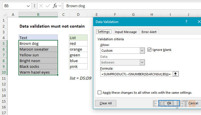
In this example, the goal is to construct a data validation rule that will prevent any one of a list of values from being entered. Data validation rules are triggered when a user adds or changes a cell value. One option is to use a formula to validate user input, which is the approach taken in the example shown, where the formula used to enforce the rule looks like this:

=SUMPRODUCT(--ISNUMBER(SEARCH(list,B5)))=0

This formula uses the SEARCH function to test user input for each value in the named range "list", which is the range D5:D10. The search logic is "contains" by default because of how SEARCH works. When a value from the "list" is found, either as a complete value or a substring, SEARCH returns the position of the match as a number. If not found, SEARCH returns an error. Since there are no invalid entries in cell B5, SEARCH returns an array of errors like this:

{#VALUE!;#VALUE!;#VALUE!;#VALUE!;#VALUE!}

The five errors tell us that no invalid entries were found. To test for invalid entries inside the formula, we use the ISNUMBER function, which returns TRUE when a value is a number and FALSE for anything else. After ISNUMBER evaluates the results from SEARCH we have an array of TRUE and FALSE values. At this point, our formula looks like this:

=SUMPRODUCT(--{FALSE;FALSE;FALSE;FALSE;FALSE})=0

Next, we use a double negative (--) to convert the TRUE and FALSE values to 1s and 0s, which yields this:

=SUMPRODUCT({0;0;0;0;0})=0

Finally, the SUMPRODUCT function sums up the items in the array and the result is tested against zero. As long as all items are zero, SUMPRODUCT returns zero and validation succeeds. If SUMPRODUCT returns a positive number, an invalid value has been found. The formula returns FALSE and validation fails.

Note: Cell references in data validation formulas are relative to the upper left cell in the range selected when the validation rule is defined, in this case, B5.