Summary
One of the most useful features of data validation is the ability to create a dropdown list that let users select a value from a predefined list. But how can you make one dropdown dynamically respond to another? In other words, how can you make the values in a dropdown list depend on another value in the worksheet? Read on to see how to create dependent dropdown lists in Excel.
Quick Links
What is a dropdown list?
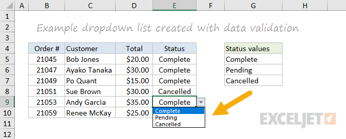
Dropdown lists allow users to select a value from a predefined list. This makes it easy for users to enter only data that meets requirements. Dropdown lists are implemented as a special kind of data validation. The screen below shows a simple example. In column E, the choices are Complete, Pending, or Cancelled, and these values are pulled automatically from the range G5:G7:
Dropdown lists are easy to create and use. But once you start to use dropdown menus in your spreadsheets, you'll inevitably run into a challenge: how can you make the values in one dropdown list depend on the values in another? In other words, how can you make a dropdown list dynamic?
Here are some examples:
- a list of cities that depends on the selected country
- a list of flavors that depends on type of ice cream
- a list of models that depends on manufacturer
- a list of foods that depends on category
These kind of lists are called dependent dropdowns, since the list depends on another value. They are created with data validation, using a custom formula based on the INDIRECT function and named ranges. This may sound complicated, but it is actually very simple, and a great example of how INDIRECT can be used.
Read on to see how to create dependent dropdown lists in Excel.
Dependent dropdown example
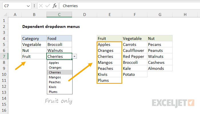
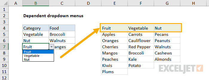
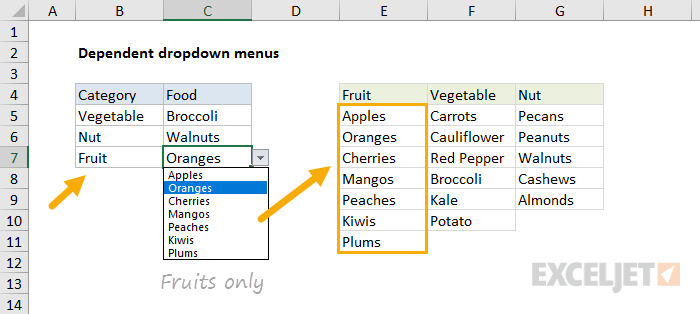
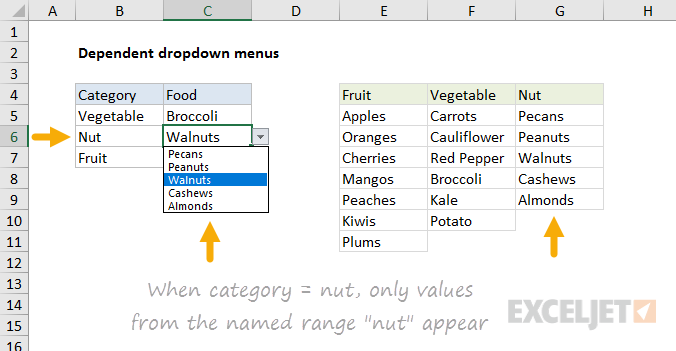
In the example shown below, column B provides a dropdown menu for food Category, and column C provides options in the chosen category. If the user selects "Fruit", they see a list of fruits, if they select "Nut", they see a list of nuts, and if they select "Vegetable", they see a list of vegetables.
The data validation in column B uses this custom formula:
=category
And the data validation in column C uses this custom formula:
=INDIRECT(B5)
Where the worksheet contains the following named ranges:
category = E4:G4
vegetable = F5:F10
nut = G5:G9
fruit = E5:E11
How this works
The key to this technique is named ranges + the INDIRECT function. INDIRECT accepts text values and tries to evaluate them as cell references. For example, INDIRECT will take the text "A1" and turn it into an actual reference:
=INDIRECT("A1")
=A1
Similarly, INDIRECT will convert the text "A1:A10" into the range A1:A10 inside another function:
=SUM(INDIRECT("A1:A10")
=SUM(A1:A10)
At first glance, you might find this construction annoying, or even pointless. Why complicate a nice simple formula with INDIRECT?
Rest assured, there is a method to the madness :)
The beauty of INDIRECT is that it lets you use text exactly like a cell reference. This provides two key benefits:
- You can assemble a text reference inside a formula, which is handy for certain kinds of dynamic references.
- You can pick up text values on a worksheet, and use them like a cell reference in a formula.
In the example on this page, we're combining the latter idea with named ranges to build dependent dropdown lists. INDIRECT maps text to a named range, which is then resolved to a valid reference. So, in this example, we're picking up the text values in column B, and using INDIRECT to convert them to cell references by matching existing named ranges, like this:
=INDIRECT(B6)
=INDIRECT("nut")
=G5:G9
B6 resolves to the text "nut" which resolves to the range G5:G9.
How to set up dependent dropdown lists
This section describes how to set up the dependent dropdown lists shown in the example.
- Create the lists you need. In the example, create a list of fruits, nuts, and vegetables in a worksheet.
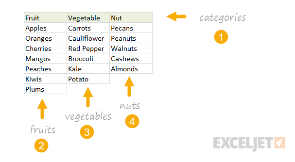
- Create named ranges for each list: category = E4:G4, vegetable = F5:F10, nut = G5:G9, and fruit = E5:E11.
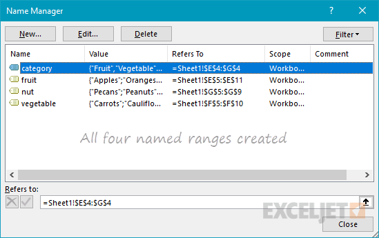
Important: the column headings in E4, F4, and G4 must match the last three named ranges above ("vegetable", "nut", and "fruit"). In other words, you must make sure that the named ranges you created match the values in the Category dropdown list.
- Create and test a data validation rule to provide a dropdown list for Category using the following custom formula:
=category
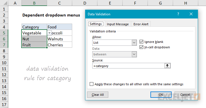
Note: just to be clear, the named range "category" is used for readability and convenience only – using a named range here is not required. Also note data validation with a list works fine with both horizontal and vertical ranges – both will be presented as a vertical dropdown menu.
- Create a data validation rule for the dependent dropdown list with a custom formula based on the INDIRECT function:
=INDIRECT(B5)
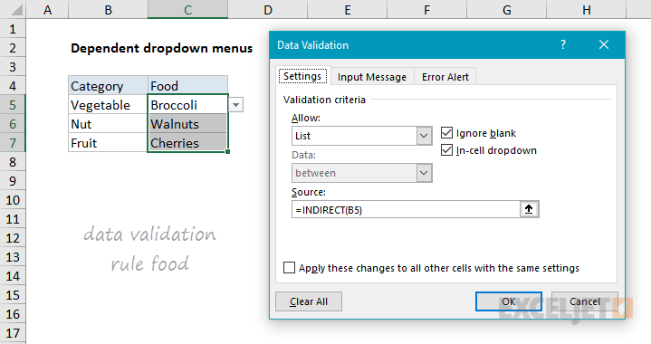
In this formula, INDIRECT simply evaluates values in column B as references, which links them to the named ranges previously defined.
- Test the dropdown lists to make sure they dynamically respond to values in column B.
Note: the approach we are taking here is not case-sensitive. The named range is called "nut" and the value in B6 is "Nut" but the INDIRECT function correctly resolves to the named range, even though case differs.
Dealing with spaces
Named ranges don't allow spaces, so the usual convention is to use underscore characters instead. So, for example, if you want to create a named range for ice cream, you would use ice_cream. This works fine, but dependent dropdown lists will break if they try to map "ice cream" to "ice_cream". To fix this problem you can use a more robust custom formula for data validation:
=INDIRECT(SUBSTITUTE(A1," ","_"))
This formula still uses INDIRECT to link the text value in A1 to a named range, but before INDIRECT runs, the SUBSTITUTE function replaces all spaces with underscores. If the text contains no spaces, SUBSTITUTE has no effect.
Practice file
The example file is attached below – check it out to see how it works. If you want to learn the technique yourself, I'd recommend you build a file of your own. The best way to learn is by doing.


