Count values out of tolerance

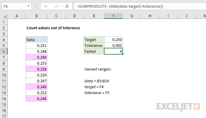
This formula counts how many values are not in range of a fixed tolerance. The variation of each value is calculated with this:

ABS(data-target)

Because the named range "data" contains 10 values, subtracting the target value in F4 will created an array with 10 results:

{0.001;-0.002;-0.01;0.003;0.008;0;-0.003;-0.01;0.002;-0.006}

The ABS function changes any negative values to positive:

{0.001;0.002;0.01;0.003;0.008;0;0.003;0.01;0.002;0.006}

This array is compared to the fixed tolerance in F5:

ABS(data-target)>tolerance

The result is an array or TRUE FALSE values, and the double negative changes these to ones and zeros. Inside SUMPRODUCT, the final array looks like this:

{0;0;1;0;1;0;0;1;0;1}

where zeros represent values within tolerance, and 1s represent values out of tolerance. SUMPRODUCT then sums the items in the array, and returns a final result, 4.

All values within tolerance

To return "Yes" if all values in a data range are within a given tolerance, and "No" if not, you can adapt the formula like this:

=IF(SUMPRODUCT(--(ABS(data-target)>tolerance)),"Yes","No")

If SUMPRODUCT returns any number greater than zero, IF will evaluate the logical test as TRUE. A zero result will be evaluated as FALSE.

Highlight values out of tolerance

You can highlight values out of tolerance with a conditional formatting rule based on a formula like this:

=ABS(B5-target)>tolerance

This page lists more examples of conditional formatting with formulas.