Summary
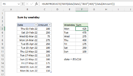
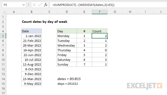
To count dates by day of the week (i.e. count Mondays, Tuesdays, Wednesdays, etc.), you can use the SUMPRODUCT function together with the WEEKDAY function. In the example shown, the formula in F5 is:
=SUMPRODUCT(--(WEEKDAY(dates,2)=E5))
where "dates" is the named range B5:B15. As the formula is copied down, it returns a count for each day shown in column D.
Generic formula
=SUMPRODUCT(--(WEEKDAY(dates)=day_num))
Explanation
You might wonder why we aren't using COUNTIF or COUNTIFS. These functions seem like the obvious solution. However, without adding a helper column that contains a weekday value, there is no way to create criteria for COUNTIF to count weekdays in a range of dates. Instead, we use the versatile SUMPRODUCT function, which handles arrays gracefully without the need to use Control + Shift + Enter. We are using SUMPRODUCT with just one argument, which consists of this expression:
--(WEEKDAY(dates,2)=E5)
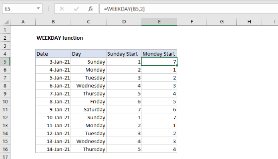
Working from the inside out, the WEEKDAY function is configured with the optional argument 2, which causes it to return numbers 1-7 for the days Monday-Sunday, respectively. This makes it easier to list the days in order with the numbers in column E in sequence. WEEKDAY evaluates each date in dates (B5:B15) and returns a number. Because we are giving WEEKDAY 11 dates, we get back an array that contains 11 results like this:
{6;1;1;6;3;7;5;6;5;3;2}
Each number in this array corresponds to a day of the week, with Mondays equal to 1 and Sundays equal to 7. Next, the numbers returned by WEEKDAY are compared to the value in E5, which is 1:
{6;1;1;6;3;7;5;6;5;3;2}=1
The result is an array of TRUE/FALSE values like this:
{FALSE;TRUE;TRUE;FALSE;FALSE;FALSE;FALSE;FALSE;FALSE;FALSE;FALSE}
In this array, TRUE corresponds to dates that fall on Monday and FALSE represents other days of the week. SUMPRODUCT only works with numbers (not text or Booleans) so we use a double-negative (--) to coerce the TRUE/FALSE values to 1s and 0s. The result is delivered directly to the SUMPRODUCT function:
=SUMPRODUCT({0;1;1;0;0;0;0;0;0;0;0}) // returns 2
With just one array to process, SUMPRODUCT sums the items and returns 2 as a final result, since there are two Mondays in the dates.
Dealing with blank dates
If you have blank cells in the list of dates, you will get incorrect results, since the WEEKDAY function will return a result even when there is no date. To handle empty cells, you can adjust the formula as follows:
=SUMPRODUCT((WEEKDAY(dates,2)=E5)*(dates<>""))
Multiplying by the expression (dates<>"") is one way to "cancel out" empty cells.
Without day numbers
The day numbers in column E make the formula easier to understand and write. However, since the day names are already in the range D5:D11, which is named days, it is possible to write a formula that doesn't use column E at all by using the MATCH function like this:
=SUMPRODUCT(--(WEEKDAY(dates,2)=MATCH(D5,days,0)))
This works because the MATCH function simply returns the position of each day name in days:
MATCH(D5,days,0) // returns 1
MATCH(D6,days,0) // returns 2
MATCH(D7,days,0) // returns 3
Otherwise, the formula works the same way and returns the same counts as the original formula.