Summary
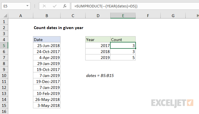
To count dates in a given year, you can use the SUMPRODUCT and YEAR functions. In the example shown, the formula in E5 is:
=SUMPRODUCT(--(YEAR(dates)=D5))
where dates is the named range B5:B15.
Generic formula
=SUMPRODUCT(--(YEAR(dates)=year))
Explanation
The YEAR function extracts the year from a valid Excel date. For example:
=YEAR("15-Jun-2021") // returns 2021
In this case, we are giving YEAR and array of dates in the named range dates:
YEAR(dates)
Because dates contains 11 cells, we get back 11 results in an array like this:
{2018;2017;2019;2019;2017;2019;2017;2019;2019;2018;2018}
Each date is compared to the year in column D, which creates a new array of TRUE FALSE values:
{FALSE;TRUE;FALSE;FALSE;TRUE;FALSE;TRUE;FALSE;FALSE;FALSE;FALSE}
In this array, TRUE corresponds to dates in the year 2017, and FALSE corresponds to dates in different years. Next, we use a double negative (--) to coerce the TRUE FALSE values to 1's and 0's. Inside SUMPRODUCT, we now have:
=SUMPRODUCT({0;1;0;0;1;0;1;0;0;0;0})
Finally, with only one array to work with, SUMPRODUCT sums the items in the array and returns a result, 3.
Note: The SUMPRODUCT formula above is an example of using Boolean logic in an array operation. This is a powerful and flexible approach to solving many problems in Excel. It is also an important skill with new functions like FILTER and XLOOKUP, which often use this technique to apply multiple criteria (FILTER example, XLOOKUP example)