=LEFT(text, [num_chars])- text - The text from which to extract characters.
- num_chars - [optional] The number of characters to extract, starting on the left. Default = 1.
Using the LEFT function
The LEFT function extracts a given number of characters from the left side of a supplied text string. The first argument, text, is the text string to extract from. This is typically a reference to a cell that contains text. The second argument, called num_chars, specifies the number of characters to extract. If num_chars is not provided, it defaults to 1. If num_chars is greater than the number of characters available, LEFT returns the entire text string. Although LEFT is a simple function, it shows up in many more advanced formulas that test or manipulate text in a specific way.
LEFT function basics
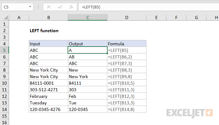
To extract text with LEFT, just provide the text and the number of characters to extract. The formulas below show how to extract one, two, and three characters with LEFT:
=LEFT("apple",1) // returns "a"
=LEFT("apple",2) // returns "ap"
=LEFT("apple",3) // returns "app"
If the optional argument num_chars is not provided, it defaults to 1:
=LEFT("ABC") // returns "A"
If num_chars exceeds the length of the text string, LEFT returns the entire string:
=LEFT("apple",100) // returns "apple"
When LEFT is used on a numeric value, the result is text:
=LEFT(1000,3) // returns "100" as text
Example - abbreviate month names
The LEFT function can be used to abbreviate text values. For example, to extract the first three characters of "January" you can use LEFT like this:
=LEFT("January",3) // returns "Jan"
Of course, it doesn't make sense to abbreviate a text string that you have to type into a formula. A more typical example is to abbreviate text values that already exist in cells, as seen in the worksheet below. The formula in cell D5, copied down, is:
=LEFT(B5,3)
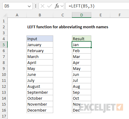
Notice num_chars is provided as 3 to extract the first 3 letters of each month.
Example - extract the first character
An interesting quirk of the LEFT function is that the number of characters to extract is not required and defaults to 1. This can be useful in cases where you only want to extract the first character of a text string, as seen below. Here, the formula in cell D5 looks like this:
=LEFT(B5)
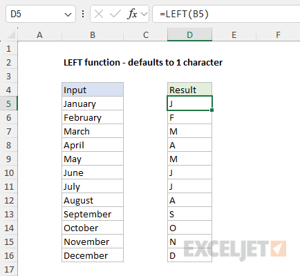
As you can see, without a value for num_chars, LEFT extracts the first letter of each month.
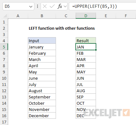
Example - LEFT with UPPER
You can easily combine LEFT with other functions in Excel to get a more specific result. For example, you could nest the LEFT function inside the UPPER function to convert the result from LEFT to uppercase. You can see this approach in the worksheet below, where the formula in cell D5 looks like this:
=UPPER(LEFT(B5,3))
Example - LEFT with IF
You can easily combine the LEFT function with the IF function to create "if cell begins with" logic. In the example below, a formula is used to flag codes that begin with "xyz" with an "x". The formula in cell D5 is:
=IF(LEFT(B5,3)="xyz","x","")
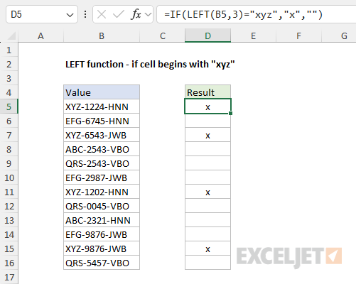
As the formula is copied down, the LEFT function returns the first 3 characters in each value, which are compared to "xyz" as a logical test. When the result is TRUE, IF returns "x". When the result is FALSE, IF returns an empty string "". The result is that the codes in column B that begin with "xyz" are clearly marked.
LEFT is not case-sensitive as you can see in the formula above. To perform a case-sensitive test you can combine LEFT with the EXACT function. Example here.
Example - LEFT with FIND
A common challenge with the LEFT function is extracting a variable number of characters, depending on the location of a specific character in the text string. To handle this situation you can use the LEFT function together with the FIND function in a generic formula like this:
=LEFT(text,FIND(character,text)-1) // extract text up to character
FIND returns the position of the character, and LEFT returns all text to the left of that position. The screen below shows how this formula can be applied in a worksheet. The formula in cell D5 is:
=LEFT(B5,FIND(" ",B5)-1)
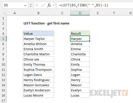
As the formula is copied down, the FIND function returns the position of the space character " " as a number. The result, minus one, is returned to the LEFT function as the num_chars argument, which then extracts all text up to the first space. You can read a more detailed explanation here.
Related functions
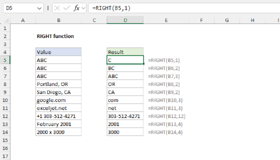
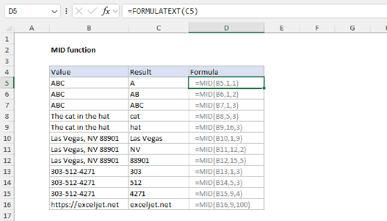
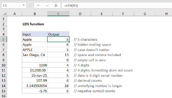
The LEFT function is used to extract text from the left side of a text string. Use the RIGHT function to extract text starting from the right side of the text, and the MID function to extract from the middle of text. The LEN function returns the length of a text string as a count of characters and is often combined with LEFT, MID, and RIGHT.
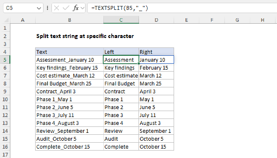
In the latest version of Excel, newer functions like TEXTBEFORE, TEXTAFTER, and TEXTSPLIT greatly simplify certain text operations and make some traditional formulas that use the LEFT function obsolete. Example here.
Notes
- LEFT is not case-sensitive.
- LEFT can extract numbers as well as text.
- The output from LEFT is always text.
- LEFT ignores number formatting when extracting characters.
- Num_chars is optional and defaults to 1.