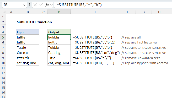
Summary
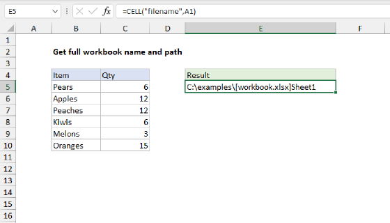
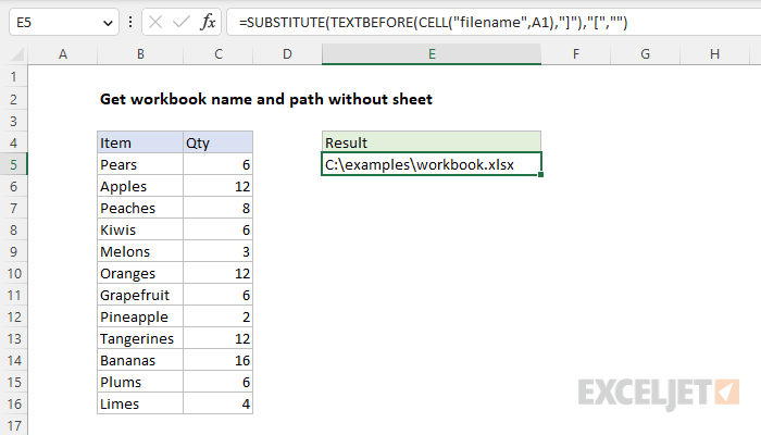
To get a path to the current workbook, you can use a formula based on the CELL function, the TEXTBEFORE function, and the SUBSTITUTE function. In the example shown, the formula in E5 is:
=SUBSTITUTE(TEXTBEFORE(CELL("filename",A1),"]"),"[","")
The result is a path and filename like this: "C:\examples\workbook.xlsx". The sheet name and the square brackets ("[ ]") that normally enclose the file name have been removed.
Generic formula
=SUBSTITUTE(TEXTBEFORE(CELL("filename",A1),"]"),"[","")
Explanation
In this example, the goal is to get a normal path to the current workbook, without a sheet name, and without the square brackets ("[ ]") that normally enclose the workbook name. This is a pretty simple problem in the latest version of Excel, which provides the TEXTBEFORE function. In older versions of Excel, you can use a more complicated formula based on the LEFT and FIND functions. Both options use the CELL function to get a full path to the current workbook. Read below for a full explanation.
Get workbook path
The first step in this problem is to get the workbook path, which includes the workbook and worksheet name. This can be done with the CELL function like this:
CELL("filename",A1)
With the info_type argument set to "filename", and reference set to cell A1 in the current worksheet, the result from CELL will be a full path as a text string like this:
"C:\path\to\folder\[workbook.xlsx]sheetname"
Notice the workbook name is enclosed in square brackets ("[name]"). This is close to what we want, but there are still two tasks that remain:
- Remove the sheet name
- Remove the square brackets ("[ ]")
The best way to do this depends on what Excel version you have. If you have the latest version of Excel, you should use a formula based on the TEXTBEFORE function. Otherwise, you can use the LEFT and FIND functions as explained below.
TEXTBEFORE option
In the worksheet shown above, the formula in E5 is:
=SUBSTITUTE(TEXTBEFORE(CELL("filename",A1),"]"),"[","")
This is an example of nesting. The CELL function is nested inside the TEXTBEFORE function, which is nested inside the SUBSTITUTE function. Working from the inside out:
- The CELL function returns the full path as a text string, as explained above.
- The TEXTBEFORE function returns all text before the closing square bracket ("]").
- The SUBSTITUTE function replaces the opening square bracket ("[") with an empty string ("").
The final result is a path to the workbook like this:
C:\path\to\folder\workbook.xlsx
Legacy Excel
In older versions of Excel without the TEXTBEFORE function, you can use a formula based on LEFT, CELL, FIND, and SUBSTITUTE:
=SUBSTITUTE(LEFT(CELL("filename",A1),FIND("]",CELL("filename",A1))-1),"[","")
At a high level, this formula works in 4 steps:
- Get the full path and filename
- Locate the closing square bracket ("]")
- Remove sheet name and "]"
- Remove the opening square bracket ("]")
Note: the CELL function is called twice in the formula because we need the path twice, once for the FIND function to locate the "]", and once for the SUBSTITUTE function to remove the "]". CELL is a volatile function and can cause performance problems in larger or more complicated worksheets.
Get path and filename
To get the path and file name, we use the CELL function like this:
CELL("filename",A1) // get path and filename
The info_type argument is "filename" and reference is A1. The cell reference is arbitrary and can be any cell in the worksheet. The result is a full path like this as text:
C:\examples\[workbook.xlsx]Sheet1
Note the sheet name("Sheet1") appears at the end.
Locate the closing square bracket
The location of the closing square bracket ("]") is calculated like this
FIND("]",CELL("filename",A1))-1 // returns 26
The FIND function returns the location of "]" (27) from which 1 is subtracted to get 26. We subtract 1 because we want to remove text starting with the "]" that follows the filename.
Remove sheet name
In the previous step, we located the "]" at character 27, then stepped back to 26. This number is returned directly to the LEFT function as the num_chars argument. The text argument is again provided by the CELL function:
LEFT("C:\examples\[workbook.xlsx]Sheet1",26)
The LEFT function returns the first 26 characters of text.
C:\examples\[workbook.xlsx
At this point, LEFT has removed the sheet name, but notice the opening square bracket "[" remains.
Remove opening square bracket
The result from LEFT is returned to the SUBSTITUTE function as the text argument:
=SUBSTITUTE("C:\examples\[workbook.xlsx","[","")
SUBSTITUTE is configured to remove the opening square bracket by setting old_text to "[" and new_text to an empty string (""). The final result returned by SUBSTITUTE is:
C:\examples\workbook.xlsx